Automated Transport Mode Detection of GPS Tracking Data

Abstract

This project aims to investigate key factors and features in GPS tracking data to differentiate transportation vehicles. Machine learning is applied to automate transportation mode detection using spatial, temporal, and attribute analysis. Manual verification of results ensures accuracy. The findings contribute to computational movement analysis and automated transportation mode detection.

1. Introduction

In recent years, the spread of GPS-enabled devices and progress in location-based technologies have generated vast amounts of GPS tracking data. This data holds significant potential for extracting insights and to improve our understanding of human mobility patterns. One main application in this field is the differentiation of transportation modes. This can benefit various domains such as traffic management or urban planning. Determining the mode of transportation from GPS tracking data presents several challenges. With the ubiquitous increase of GPS tracking through smartphones and other technical devices, it’s too time consuming and expensive to manually annotate data and also prone to human error or biases. This leads to the following two research questions:

What are the key factors and features that can be extracted from GPS tracking data to differentiate between different types of transportation modes?

How can machine learning techniques be applied to GPS tracking data to automate the detection of the mode of transportation and which accuracies can be achieved by different machine learning algorithms?

The project will focus on exploring spatial and temporal aspects to extract key factors from GPS tracking data, such as velocity, sinuosity or angles. Additionally, spatial context in the form of traffic networks and land cover is added to the data in order to improve the accuracy of transportation mode detection. Machine learning algorithms will be tested and employed to automate the classification of transportation modes. An accurate algorithm is aimed to be found by training and evaluating different models on labeled data. These models include random forests, support vector machines or neural networks. To ensure the accuracy of the models, a subset of the classified data is used to validate the performance. By comparing the results of the automated classification with ground truth data, the project aims to assess the achieved accuracies of different machine learning algorithms and identify areas for improvement.

2. Data

The main data are the GPS tracking data, which were recorded through the Posmos App via smartphone throughout a time span of approximately 1.5 months by the two authors and from the available data pool. The complete collected data was manually labelled to ensure a valid ground truth. Further, spatial context data such as the Swiss road network, tram network,¹ train network² and the bus network of the cantons of Zurich³ and Bern.⁴ (Note: There is no official data set for the entire Swiss bus network according to the federal bureau of transport. Thus the available ones for Bern and Zurich were used, where a significant amount of data points pertaining to bus usage were collected). To facilitate the detection of the transportation mode boat, land cover data containing all Swiss waters was also used.⁵

Code

library("dplyr")
library("sf")
library("readr") 
library("ggplot2")
library("mapview")
library("lubridate")
library("zoo") 
library("caret")
library("LearnGeom") # to calculate angle
library("geosphere") # to calculate distances
library("RColorBrewer") # to create custom color palette
library("ggcorrplot") # for correlation matrix
library("ROSE")
library("gridExtra")

Code

# creates lines out of points, used for visualisation purposes
point2line <- function(points){
  geometries <- st_cast(st_geometry(points %>% select(geometry)), "POINT")
  n <- length(geometries) - 1
  linestrings <- lapply(X = 1:n, FUN = function(x) {

  pair <- st_combine(c(geometries[x], geometries[x + 1]))
  line <- st_cast(pair, "LINESTRING")
  return(line)
  })
  
  multilinetring <- st_multilinestring(do.call("rbind", linestrings))
  
  df <- data.frame(linestrings[1])
  
  for (i in 2:length(linestrings)){
    temp <- data.frame(linestrings[i])
    df <-  rbind(df, temp) 
  }
  sf_lines <- df %>% st_as_sf()
}

un_col <- function(df){
  return(length(unique(df)))
}

Code

# read personal tracking data
posmo_micha_truth_csv <- read.delim("data/manually_labelled/posmo_20230502_to_20230613_m.csv",sep=",") 
posmo_cyril_truth_csv <- read.delim("data/manually_labelled/posmo_2023-05-01T00_00_00+02_00-2023-06-26T23_59_59+02_00.csv",sep=",") 
posmo_micha_csv <- read.delim("data/posmo_labelled/posmo_20230502_to_20230613_p.csv",sep=",") 


# read tracking data from pool
posmo_pool_1 <- read.delim("data/manually_labelled/posmo.csv",sep=",") %>% tail(612) # last 250 data points are not correctly labelled
posmo_pool_2 <- read.delim("data/manually_labelled/posmo_2.csv",sep=",") 
posmo_pool_3 <- read.delim("data/manually_labelled/posmo_BuJa.csv",sep=",") 

Code

# read context data
tram_netz <- read_sf("data/tlm_oev_eisenbahn/tlm_oev_eisenbahn_tram.shp") %>%
  select(id, geometry) %>% st_zm() %>% st_buffer(10) %>% st_union
zug_netz <- read_sf("data/tlm_oev_eisenbahn/tlm_oev_eisenbahn_bahn.shp") %>% 
  select(id, geometry) %>% st_zm() %>% st_buffer(10) %>% st_union
gewaesser <- read_sf("data/tlm_bb_gewaesser/tlm_bb_gewaesser_larger20000.shp") %>% 
  select(id, geometry) %>% st_zm() %>% st_union
strassen <- read_sf("data/tlm_strassen/strassen_AOI.shp") %>% 
  select(id, geometry) %>% st_zm() %>% st_buffer(10) %>% st_union

bus_netz_zvv <- read_sf("data/zvv_netz/Linien_des_offentlichen_Verkehrs_-OGD.gpkg", layer="ZVV_LINIEN_L")
bus_netz_zvv <- bus_netz_zvv[grepl("bus|Bus", bus_netz_zvv$BETRIEBSZWEIG_TXT), ] %>% rename(geometry = geom) %>%
  select(geometry) %>% st_buffer(10) %>% st_union()

bus_netz_bern <- read_sf("data/geoinformation_bern/OEVTP_LINIE.shp") %>% filter(VERKMITT_B == "Bus") %>% select(geometry) %>%st_zm() %>% st_buffer(10) %>% st_union()

bus_netz <- st_union(bus_netz_bern, bus_netz_zvv)

Code

process_posmo_data <- function(posmo_data) { # function with data cleaning steps

  # Convert to sf object
  posmo_data <- posmo_data %>%
    st_as_sf(coords = c("lon_x", "lat_y"), crs = 4326) %>%
    st_transform(crs = 2056)
  
  # Remove unwanted columns
  posmo_data <- posmo_data[, -c(1, 3, 4)]
  
  # Fix Timestamp
  posmo_data$datetime <- ymd_hms(posmo_data$datetime) + hours(2)
  
  # Add ID to rows
  posmo_data <- posmo_data %>%
    mutate(id = row_number())
  
  # remove duplicate time values
  posmo_data <- posmo_data[!duplicated(posmo_data$datetime), ]
  
  # remove subsequent duplicate location (person wasn't moving)
  posmo_data <- posmo_data %>% 
    filter(geometry != lead(geometry))
  
  return(posmo_data)
}

3. Methods

3.1 Preprocessing

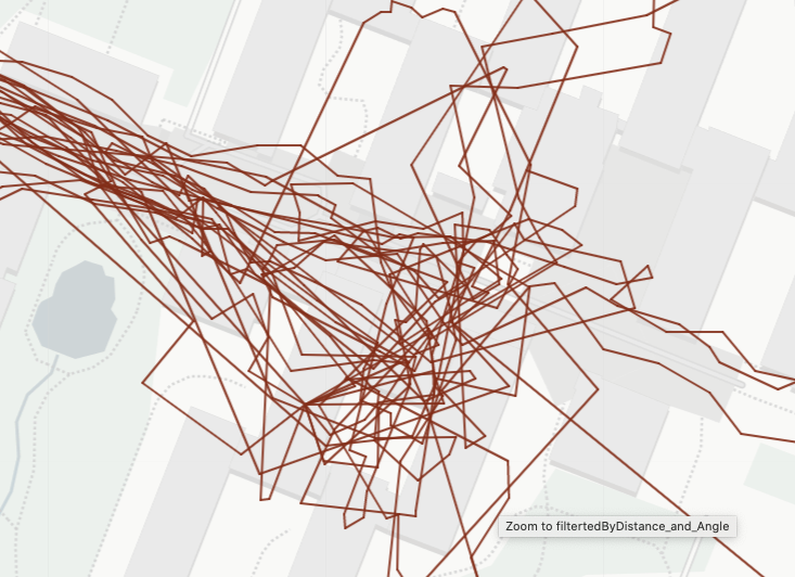
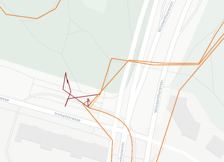
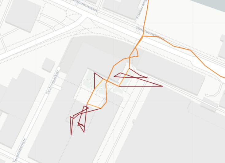
When tracking a person throughout the day using GPS data, there are instances where the person appears to be stationary, such as when in an office or at a university. However, due to GPS inaccuracies, these stationary points may not appear at the exact same location and can exhibit erratic movement patterns. The accuracy of GPS signals is often compromised in dense buildings, amplifying this phenomenon. The figure below shows an example of this phenomenon around the Irchel campus of the University of Zurich.

As a result, parameters like velocity and step length can show values that are typically associated with other categories. To address this issue, two approaches have been employed.

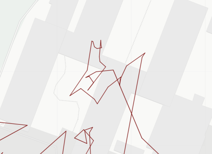
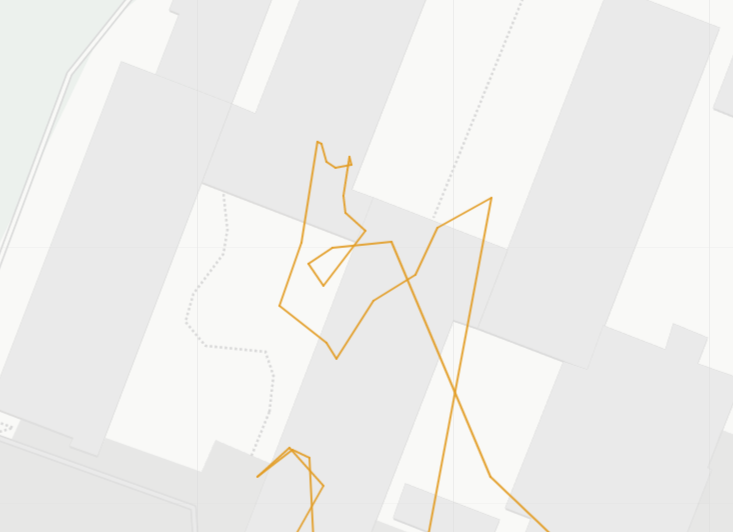
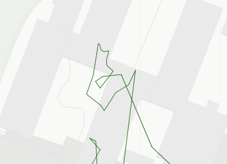
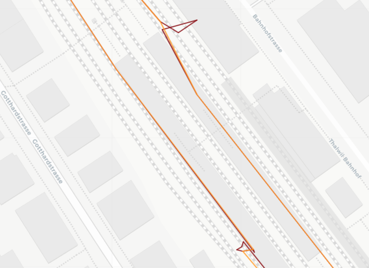
The first approach involves analyzing the angles between consecutive points. Typically, these angles are significantly smaller for stationary points compared to other movements. By visually determining a threshold angle the data set is filtered to remove all data points with angles smaller than 60°. This process needs to be repeated iteratively until no angles below the threshold remain, as the removal of data points alters the angles between the remaining points. The figure below shows the first three iterations of this process, removing more and more points with angles below the threshold.

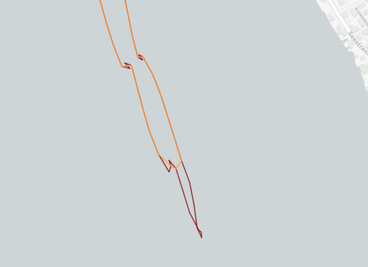
In certain situations, small angles can occur naturally and are not indicative of errors. However, the current approach of removing points based on angle thresholds may mistakenly eliminate these valid data points. This becomes particularly problematic when dealing with sharp changes in direction, such as U-turns or sudden turns. When a sharp change in direction occurs, the angle between the points just before and after the turn may be small, potentially triggering the removal of these points. As a consequence, the removal of these points alters the data set, requiring the recalculation of angles. This subsequent recalculation can lead to the removal of additional points and the inadvertent loss of significant segments of data. The figures below illustrate this phenomenon.

However, through visual inspection of a representative amount of data, it appeared that this only occurs rarely.

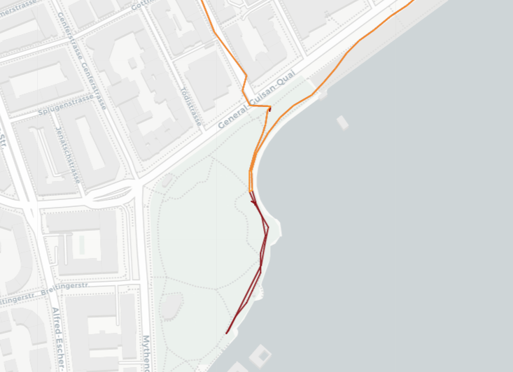
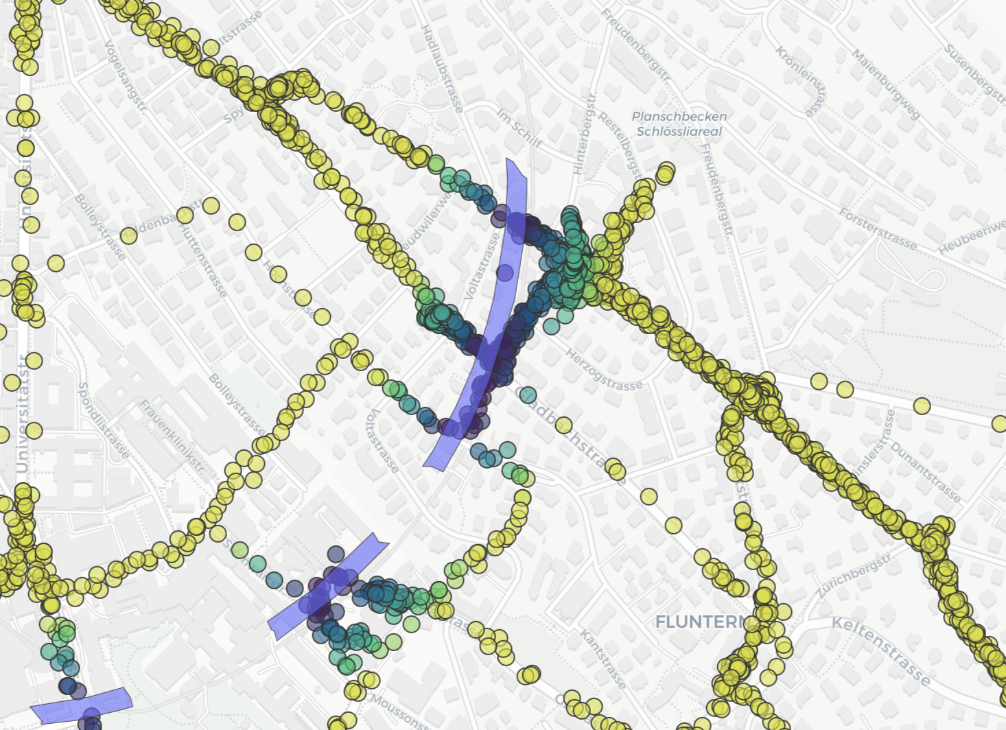
The second approach considers the distance between the current point and a set number of preceding and consecutive points. A point is deemed static if the maximum distance between that point and any of the set number of preceding or consecutive points exceeds a predefined distance threshold. However, this approach may unintentionally remove non-static data points, particularly when a person is walking slowly and numerous data points are recorded within a small distance. Adjusting the distance threshold or the number of preceding and consecutive points can mitigate this issue, but it requires striking a balance between filtering out false movements and retaining genuine data. The sampling rate of Posmos was set to 10 or 15 seconds, but in some cases, data points were recorded every three seconds. Obviously, this enhances the the chances of removing data in the just described way. Since this behavior was not expected and only discovered late in the process, the point exhibiting an abnormally short sampling interval were not removed prior to preprocessing.

Finding the optimal compromise between these filtering approaches involves considering the specific characteristics of the tracked person’s movements and the quality of the GPS data. By iteratively applying the angle-based filtering and analyzing the distance to surrounding points, a more accurate identification of stationary periods can be achieved, mitigating the impact of GPS inaccuracies and preserving the integrity of the tracking data. Thus, the thresholds were set by trial and error.

The figures below show before/after visualizations of this process.

Code

filterStaticByDistance <- function(data, threshold_distance, consecutive_points) {
  require(geosphere)
  
  # transform to WGS84, necessary to calculate distance using geosphere
  data <- data %>% st_transform(4326)
  
  # Extract coordinates from the geometry
  coords <- data.frame(st_coordinates(data))
  data$longitude <- coords$X
  data$latitude <- coords$Y
  
  # Calculate distances to preceding and consecutive points
  distances <- numeric(nrow(data))
  for (i in (consecutive_points + 1):(nrow(data) - consecutive_points)) {
    next_points <- coords[(i + 1):(i + consecutive_points), ]
    prev_points <- coords[(i - 1):(i - consecutive_points), ]
    all_points <- rbind(next_points, prev_points)
    distances[i] <- max(geosphere::distGeo(coords[i, ], all_points))
  }
  
  # Filter out points where the maximum distance exceeds the threshold
  filtered_data <- data[distances >= threshold_distance | distances == 0, ] # keep first/last values which are 0
  
  # Transform back to LV95
  filtered_data <- filtered_data %>% st_transform(2056)
  
  return(list(filtered_data = filtered_data, distances = distances)) # distances are just needed for testing thresholds
}

Code

getAngle <- function(coords) {
  angles <- numeric(nrow(coords)) # Initialize angles as a numeric vector
  angles[1] = NA # first point can't have an angle

  for (i in 2:(nrow(coords) - 1)) { # calculate the angle for 3 consecutive points, similar to lag/lead
    angle <- Angle( #function from library LearnGeom
      c(coords[i - 1, "X"], coords[i - 1, "Y"]),
      c(coords[i, "X"], coords[i, "Y"]),
      c(coords[i + 1, "X"], coords[i + 1, "Y"])
    )
    angles[i] <- angle # Assign the calculated angle to the corresponding index in angles
  }
  angles[nrow(coords)] = NA # last point cant have an angle
  return(c(angles))
}

Code

filterStaticByAngle <- function(working_dataset, angleTreshold){
  coords <- data.frame(st_coordinates(working_dataset), working_dataset$id)  
  working_dataset$angle <- getAngle(coords)
  min_angle <- min(working_dataset$angle, na.rm = T)


  while (min_angle <= angleTreshold) { # iteratively filter out tight angles until none smaller 60 are left
    working_dataset <- working_dataset %>% filter(is.na(angle) | angle > angleTreshold) # exclude first and last value (=NA)
    coords <- data.frame(st_coordinates(working_dataset), working_dataset$id)
    working_dataset$angle <- getAngle(coords)
    min_angle <- min(working_dataset$angle, na.rm = T)
  }
  return(working_dataset)
}

3.2 Movement Parameters

As variables for the machine learning models the following movement parameters have been calculated:

• Step length

• Velocity

• Acceleration

• Time difference

• Sinuosity

• Angle

Code

calc_movement_params <- function(working_dataset){

  # Create Coord Column
  coords <- data.frame(st_coordinates(working_dataset), working_dataset$id)

  # Calculate Time Difference between steps (diff_s), steplenght and velocity. 
  working_dataset <- working_dataset |> 
  mutate(diff_s = as.numeric(difftime(lead(datetime),datetime))) |>
  mutate(steplength = ((coords$X - lead(coords$X))^2 + (coords$Y - lead(coords$Y))^2)^0.5) |>
  mutate(velocity = as.numeric(steplength/diff_s)) |>
  filter(diff_s != 0)

  coords <- data.frame(st_coordinates(working_dataset), working_dataset$id)
  
  #Calculate Moving Window Step length
  working_dataset <- working_dataset |>
  mutate(
    step_mean = rowMeans(
      cbind(
        sqrt((lag(coords$X, 3) - coords$X)^2 + (lag(coords$Y, 3) - coords$Y)^2),
        sqrt((lag(coords$X, 2) - coords$X)^2 + (lag(coords$Y, 2) - coords$Y)^2),
        sqrt((lag(coords$X, 1) - coords$X)^2 + (lag(coords$Y, 1) - coords$Y)^2),
        sqrt((coords$X - lead(coords$X, 1))^2 + (coords$Y - lead(coords$Y, 1))^2),
        sqrt((coords$X - lead(coords$X, 2))^2 + (coords$Y - lead(coords$Y, 2))^2),
        sqrt((coords$X - lead(coords$X, 3))^2 + (coords$Y - lead(coords$Y, 3))^2)
      )
    )
  )
  
  #Calculate Moving Window diff_s
  working_dataset <- working_dataset |>
  mutate(diff_s_mean = as.numeric(difftime(lead(datetime,3),lag(datetime,3)))/6)

  #Calculate Moving Window velocity
  working_dataset <- working_dataset |>
  mutate(velocity_mean = as.numeric(step_mean/diff_s_mean))
 
  # Delete Infitinte Values (is there better solution?)
  #working_dataset$velocity <- working_dataset$velocity[!is.infinite(working_dataset$velocity)]
  coords <- data.frame(st_coordinates(working_dataset), working_dataset$id)

  #Acceleration stepwise
  working_dataset$acceleration <- working_dataset$velocity/lag(working_dataset$diff_s)

  # Calculate acceleration using a moving window
  working_dataset <- working_dataset |>
  mutate(
    acceleration_mean = rowMeans(
      cbind(
        lag(working_dataset$acceleration,3),
        lag(working_dataset$acceleration,2),
        lag(working_dataset$acceleration,1),
        working_dataset$acceleration,
        lead(working_dataset$acceleration,1),
        lead(working_dataset$acceleration,2),
        lead(working_dataset$acceleration,3)
      )
    )
  )
  
  # Calculate Sinuosity using moving step_mean as path length and euclidean distance between
  working_dataset <- working_dataset |>
  mutate(
    sinuosity = 
      ( # Path Length/Direct distance between first and last point
        sqrt((lag(coords$X, 3) - lag(coords$X, 2))^2 + (lag(coords$Y, 3) - lag(coords$Y, 2))^2) +
        sqrt((lag(coords$X, 2) - lag(coords$X, 1))^2 + (lag(coords$Y, 2) - lag(coords$Y, 1))^2) +
        sqrt((lag(coords$X, 1) - coords$X)^2 + (lag(coords$Y, 1) - coords$Y)^2) +
        sqrt((coords$X - lead(coords$X, 1))^2 + (coords$Y - lead(coords$Y, 1))^2) +
        sqrt((lead(coords$X, 1) - lead(coords$X, 2))^2 + (lead(coords$Y, 1) - lead(coords$Y, 2))^2) +
        sqrt((lead(coords$X, 2) - lead(coords$X, 3))^2 + (lead(coords$Y, 2) - lead(coords$Y, 3))^2)
      ) 
      / sqrt((lag(coords$X, 3) - lead(coords$X, 3))^2 + (lag(coords$Y, 3) - lead(coords$Y, 3))^2)
  ) 

  return(working_dataset)
}

Code

run_all <- function(df){
  df <- process_posmo_data(df)
  result <- filterStaticByDistance(df, threshold_distance = 60, consecutive_points = 5)
  result$filtered_data
  filtered_by_angle <- filterStaticByAngle(result$filtered_data, 60)
  df <- calc_movement_params(filtered_by_angle)
  return(df)
}

Code

working_dataset <- run_all(posmo_micha_truth_csv)
processed_1 <- run_all(posmo_cyril_truth_csv)
processed_2 <- run_all(posmo_pool_1)
processed_3 <- run_all(posmo_pool_2)
processed_4 <- run_all(posmo_pool_3)

# Combine data sets
working_dataset <- rbind(working_dataset, processed_1)
posmo_pool <- rbind(processed_2,processed_3,processed_4)

3.3 Contextual Data

Due to similar movement parameters for transportation modes it is a particularly challenging task to automatically classify transportation modes using only movement parameters. Bus and tram in cities for example, exhibit very similar characteristics. To facilitate the classification task, the data was enriched with spatial context data in the form of various networks and land cover, as mentioned in the data description. By incorporating this spatial context data, the classification process can be enhanced by considering the surrounding environment in which the transportation modes operate. For every data point, the closest distance to the difference networks and water bodies was calculated. In some cases, the calculated distances to these networks or water bodies could be extremely large. Including such large values in the data set would lead to a significant span of values, potentially overshadowing smaller differences within cities. To avoid this issue, a decision was made to set a maximum distance of 100m. Any distance beyond 100m was assigned a value of 100m. By setting this threshold, the data set ensures that distances beyond 100m are treated as equal, effectively reducing the influence of extremely large distances on the classification task.

It is important to note that the distance calculation in the data set may not always provide an accurate representation of real distances, especially in cases involving tunnels or underground passages with overlaying data points. An example of this can be seen below, where a tunnel leads close underneath the house of one of the authors and wrong distance proximites are calculated. (Side note: For processing reasons, the networks were intersected with the data points, prior to the distance calculations, that’s why only these parts of the tunnel are visible)

Code

# since some of the networks are extremly large data sets, a buffer of all data points were intersected with the networks, and only the network segments that intersected were used to calculate the distance. this was done once and then written as data set, so that this doesnt have to be computed every time
#data_AOI <- st_buffer(working_dataset, 50) %>% st_union()

tram_netz_AOI <- read_sf("processed_data/tram_netz_AOI.shp")
bus_netz_AOI <- read_sf("processed_data/bus_netz_AOI.shp")
zug_netz_AOI <- read_sf("processed_data/zug_netz_AOI.shp")
gewaesser_AOI <- read_sf("processed_data/gewaesser_AOI.shp")
strassen <- read_sf("processed_data/strassen.shp")

#tram_netz_AOI <- st_intersection(tram_netz, data_AOI)
working_dataset$distance_tram <- as.numeric(st_distance(working_dataset, tram_netz_AOI))
working_dataset$distance_tram <- ifelse(working_dataset$distance_tram > 100, 100, working_dataset$distance_tram)

#zug_netz_AOI <- st_intersection(zug_netz, data_AOI)
working_dataset$distance_zug <- as.numeric(st_distance(working_dataset, zug_netz_AOI))
working_dataset$distance_zug <- ifelse(working_dataset$distance_zug > 100, 100, working_dataset$distance_zug)

#gewaesser_AOI <- st_intersection(gewaesser, data_AOI)
working_dataset$distance_gewaesser <- as.numeric(st_distance(working_dataset, gewaesser_AOI))
working_dataset$distance_gewaesser <- ifelse(working_dataset$distance_gewaesser > 100, 100, working_dataset$distance_gewaesser)

#bus_netz_AOI <- st_intersection(bus_netz, data_AOI)
working_dataset$distance_bus <- as.numeric(st_distance(working_dataset, bus_netz_AOI))
working_dataset$distance_bus <- ifelse(working_dataset$distance_bus > 100, 100, working_dataset$distance_bus)

working_dataset$distance_strasse <- as.numeric(st_distance(working_dataset, strassen))
working_dataset$distance_strasse <- ifelse(working_dataset$distance_strasse > 100, 100, working_dataset$distance_strasse)

Code

data_AOI <- st_buffer(posmo_pool, 50) %>% st_union()

#tram_netz_AOI <- st_intersection(tram_netz, data_AOI)
posmo_pool$distance_tram <- as.numeric(st_distance(posmo_pool, tram_netz_AOI))
posmo_pool$distance_tram <- ifelse(posmo_pool$distance_tram > 100, 100, posmo_pool$distance_tram)

#zug_netz_AOI <- st_intersection(zug_netz, data_AOI)
posmo_pool$distance_zug <- as.numeric(st_distance(posmo_pool, zug_netz_AOI))
posmo_pool$distance_zug <- ifelse(posmo_pool$distance_zug > 100, 100, posmo_pool$distance_zug)

#gewaesser_AOI <- st_intersection(gewaesser, data_AOI)
posmo_pool$distance_gewaesser <- as.numeric(st_distance(posmo_pool, gewaesser_AOI))
posmo_pool$distance_gewaesser <- ifelse(posmo_pool$distance_gewaesser > 100, 100, posmo_pool$distance_gewaesser)

#bus_netz_AOI <- st_intersection(bus_netz, data_AOI)
posmo_pool$distance_bus <- as.numeric(st_distance(posmo_pool, bus_netz_AOI))
posmo_pool$distance_bus <- ifelse(posmo_pool$distance_bus > 100, 100, posmo_pool$distance_bus)

posmo_pool$distance_strasse <- as.numeric(st_distance(posmo_pool, strassen))
posmo_pool$distance_strasse <- ifelse(posmo_pool$distance_strasse > 100, 100, posmo_pool$distance_strasse)

Code

# Replace NA values with a specified value (e.g., mean, median, or 0)

working_dataset$sinuosity[is.infinite(working_dataset$sinuosity)] <- NA
working_dataset <- na.omit(working_dataset)

posmo_pool$sinuosity[is.infinite(posmo_pool$sinuosity)] <- NA
posmo_pool <- na.omit(posmo_pool)

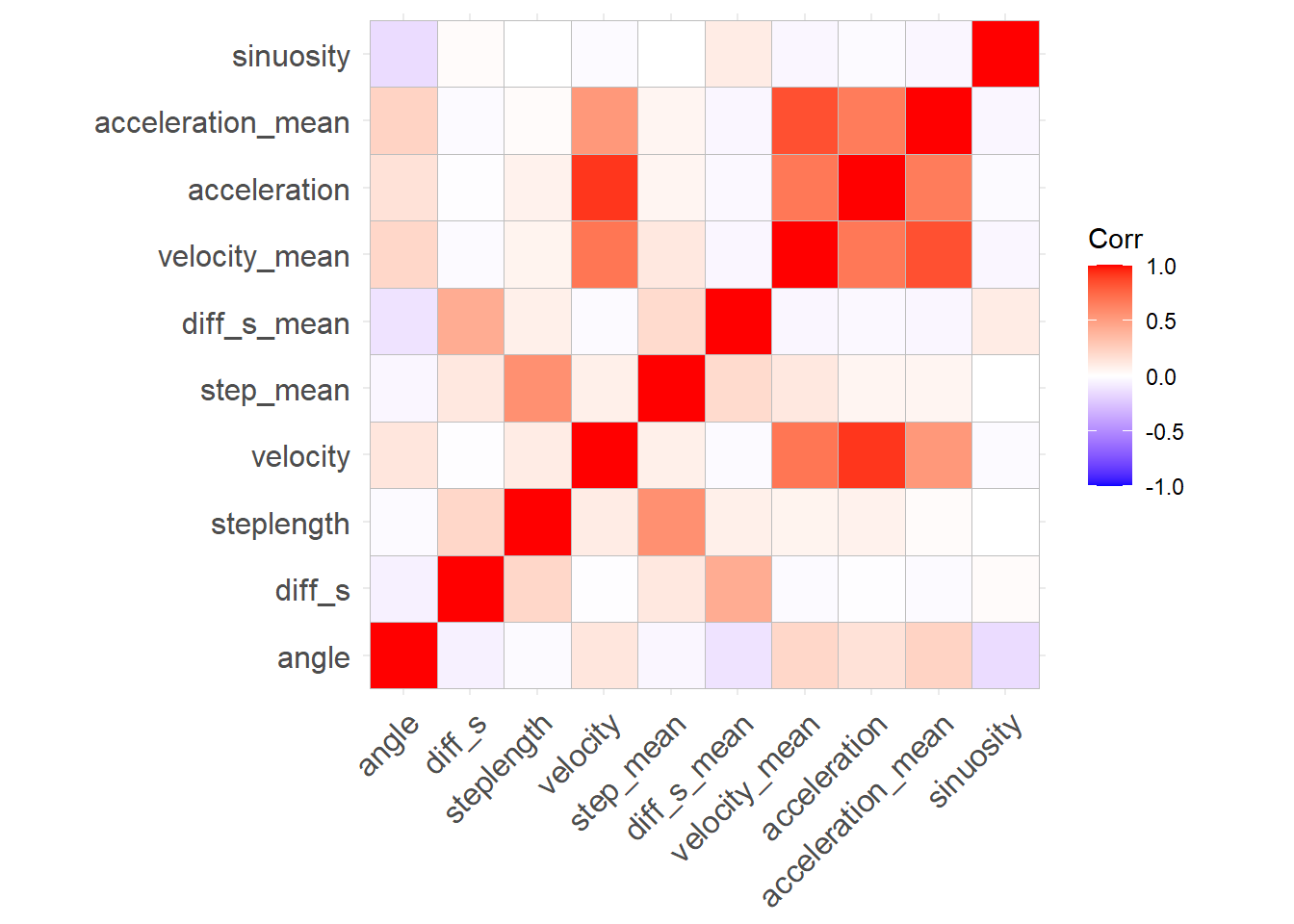
3.4 Variable Correlation

The correlation matrix shows correlation between variables. Computed velocities and acceleration correlate strongly. Other variables show only little correlation.

Code

# select columns with relevant variable and standardize them
standardized <- working_dataset[, 6:15] %>% 
  st_drop_geometry() %>%
  scale(center = TRUE, scale = TRUE) %>%
  as.data.frame()


corr_matrix <- cor(standardized)
ggcorrplot(corr_matrix)

Code

data_pca <- princomp(corr_matrix)
loadings <- data_pca$loadings
scores <- as.data.frame(data_pca$scores)

Code

# Save full dataset as csv
working_dataset <- st_drop_geometry(working_dataset)
posmo_pool <- st_drop_geometry(posmo_pool)

write.csv(working_dataset, file = "data/full_working_dataset.csv", row.names = F)
write.csv(posmo_pool, file = "data/full_posmo_pool_dataset.csv", row.names = F)

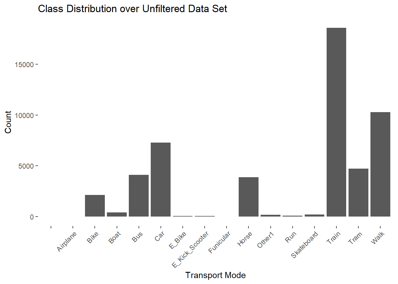
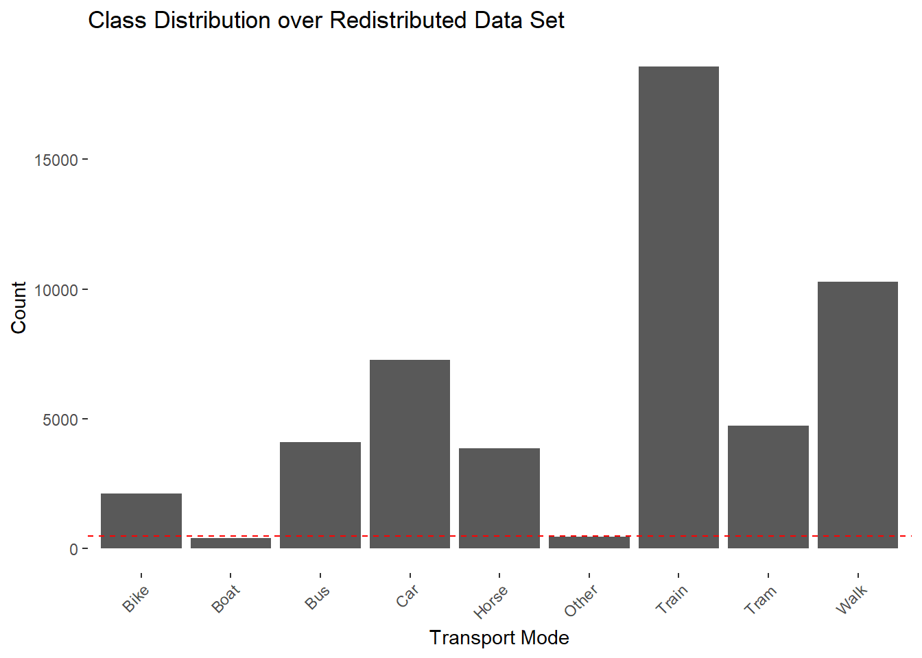
3.5 Class Distribution Overview

Code

working_dataset <- read.delim("data/full_working_dataset.csv",sep=",", header = T) 
posmo_pool <- read.delim("data/full_posmo_pool_dataset.csv",sep=",", header = T) 

working_dataset <- rbind(working_dataset, posmo_pool)

working_dataset <- na.omit(working_dataset)
# Show class distribution
ggplot(working_dataset) + 
  geom_bar(aes(x = transport_mode)) +
  theme(axis.text.x = element_text(angle = 45, hjust = 1)) +
  ggtitle("Class Distribution over Unfiltered Data Set") +
  xlab("Transport Mode") + ylab("Count")

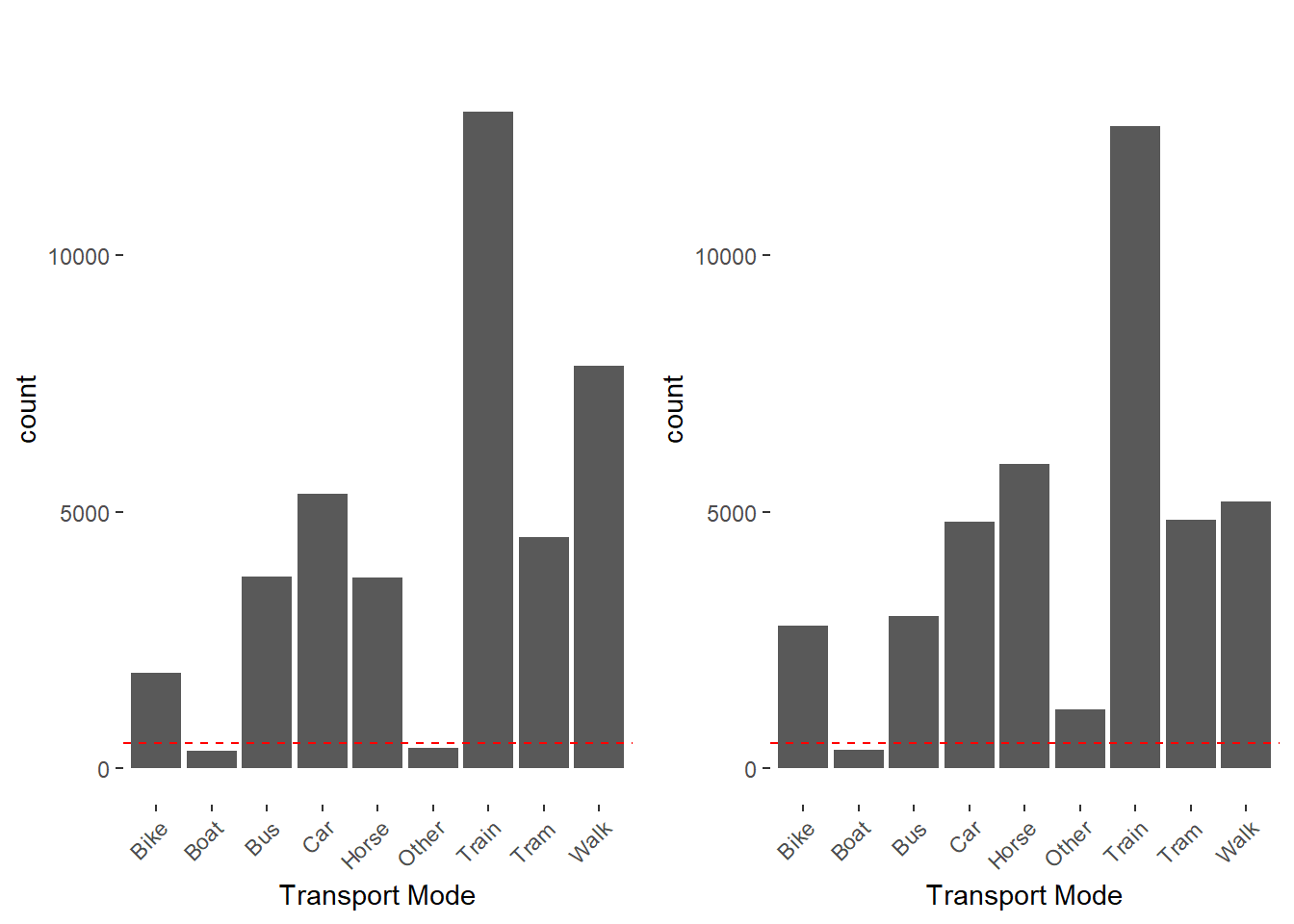
The distribution shows that many classes are very poorly represented in the data. Unclassified data is removed and aggregated. The underrepresented transport modes are moved to the class “Other”.

Code

# Remove unwanted classes
working_dataset <- working_dataset[working_dataset$transport_mode != "", ]
working_dataset <- working_dataset[working_dataset$transport_mode != "Other1", ]
# working_dataset <- working_dataset[working_dataset$transport_mode != "Funicular", ]
# working_dataset <- working_dataset[working_dataset$transport_mode != "E_Kick_Scooter", ]
# working_dataset <- working_dataset[working_dataset$transport_mode != "Run", ]
# working_dataset <- working_dataset[working_dataset$transport_mode != "Boat", ]
# working_dataset <- working_dataset[working_dataset$transport_mode != "Skateboard", ]

# Move less relevant modes into category "other"
working_dataset$transport_mode[working_dataset$transport_mode == "Funicular"] <- "Other"
working_dataset$transport_mode[working_dataset$transport_mode == "E_Kick_Scooter"] <- "Other"
working_dataset$transport_mode[working_dataset$transport_mode == "Run"] <- "Other"
working_dataset$transport_mode[working_dataset$transport_mode == "Skateboard"] <- "Other"
working_dataset$transport_mode[working_dataset$transport_mode == "Airplane"] <- "Other"
working_dataset$transport_mode[working_dataset$transport_mode == "E_Bike"] <- "Other"
# working_dataset$transport_mode[working_dataset$transport_mode == "Boat"] <- "Other"

# Show class distribution
classes <- ggplot(working_dataset) + 
  geom_bar(aes(x = transport_mode)) +
  theme(axis.text.x = element_text(angle = 45, hjust = 1)) +
  geom_hline(yintercept = 500, colour = "red", linetype = "dashed") +
  ggtitle("Class Distribution over Redistributed Data Set") +
  xlab("Transport Mode") + ylab("Count")

classes

Code

table(working_dataset$transport_mode)

 Bike  Boat   Bus   Car Horse Other Train  Tram  Walk 
 2120   417  4100  7272  3866   468 18581  4732 10281 

The dotted red line lies at a count of 500, representing the desired sample count for the following under sampling of our data set.

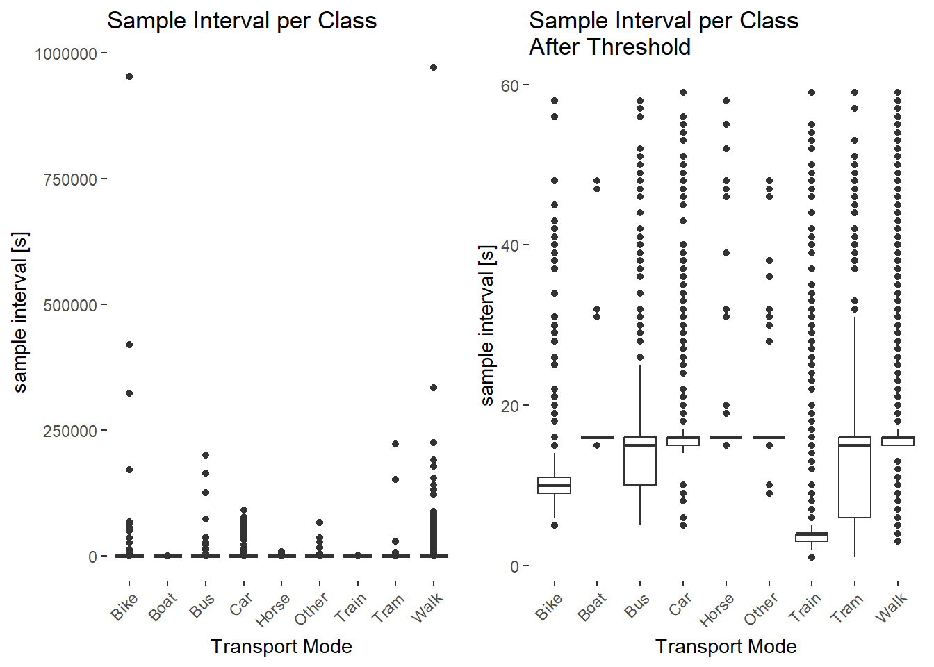
3.6 Sampling Interval

The sampling intervals were found to be highly inconsistent. Many large sampling intervals originate from the tracked person being stationary. Therefore the sampling interval is limited to 60 seconds. No re-sampling to equalize the sampling interval is undertaken, to preserve the GPS position and the calculated parameters for each data point, since with large sampling intervals the calculated movement parameters become inaccurate and unrepresentative of the transport mode. After applying the threshold the actual sampling interval of 10, respective 15 seconds can be seen in the box plot.

Code

boxplot_diff_s <- ggplot(working_dataset,aes(x = transport_mode, y = diff_s)) +
  geom_boxplot() +
  theme(axis.text.x = element_text(angle = 45, hjust = 1)) +
  ylab("sample interval [s]") + xlab("Transport Mode") +
  ggtitle("Sample Interval per Class")

# Set threshold for parameters
working_dataset <- working_dataset[working_dataset$diff_s < 60,]

boxplot_diff_s_after <- ggplot(working_dataset, aes(x = transport_mode, y = diff_s)) + 
  geom_boxplot() +
  theme(axis.text.x = element_text(angle = 45, hjust = 1)) +
  ylab("sample interval [s]") + xlab("Transport Mode") +
  ggtitle("Sample Interval per Class \nAfter Threshold")

# Display the plots side by side
grid.arrange(boxplot_diff_s, boxplot_diff_s_after, nrow = 1)

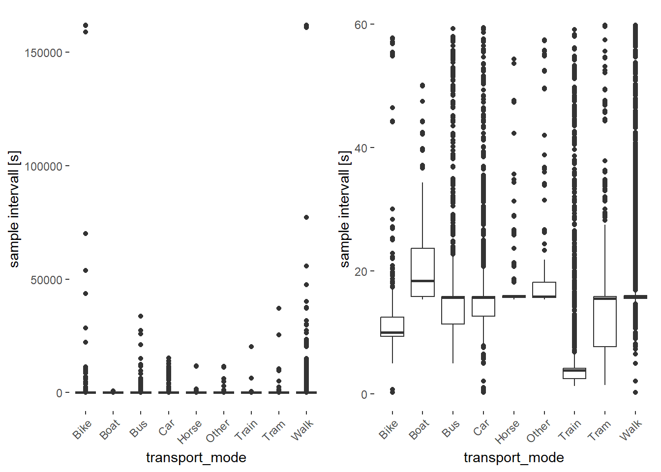
After the initial removal of sampling intervals larger than 60 seconds the step for the moving window sampling intervals is repeated.

Code

boxplot_diff_s_mean <- ggplot(working_dataset, aes(x = transport_mode, y = diff_s_mean)) +
  geom_boxplot() +
  theme(axis.text.x = element_text(angle = 45, hjust = 1)) +
  ylab("sample intervall [s]")

# Set threshold for parameters
working_dataset <- working_dataset[working_dataset$diff_s_mean < 60,]

boxplot_diff_s_mean_after <- ggplot(working_dataset, aes(x = transport_mode, y = diff_s_mean)) +
  geom_boxplot() +
  theme(axis.text.x = element_text(angle = 45, hjust = 1)) +
  ylab("sample intervall [s]")

# Display the plots side by side
grid.arrange(boxplot_diff_s_mean, boxplot_diff_s_mean_after, nrow = 1)

3.7 Parameter Thresholds

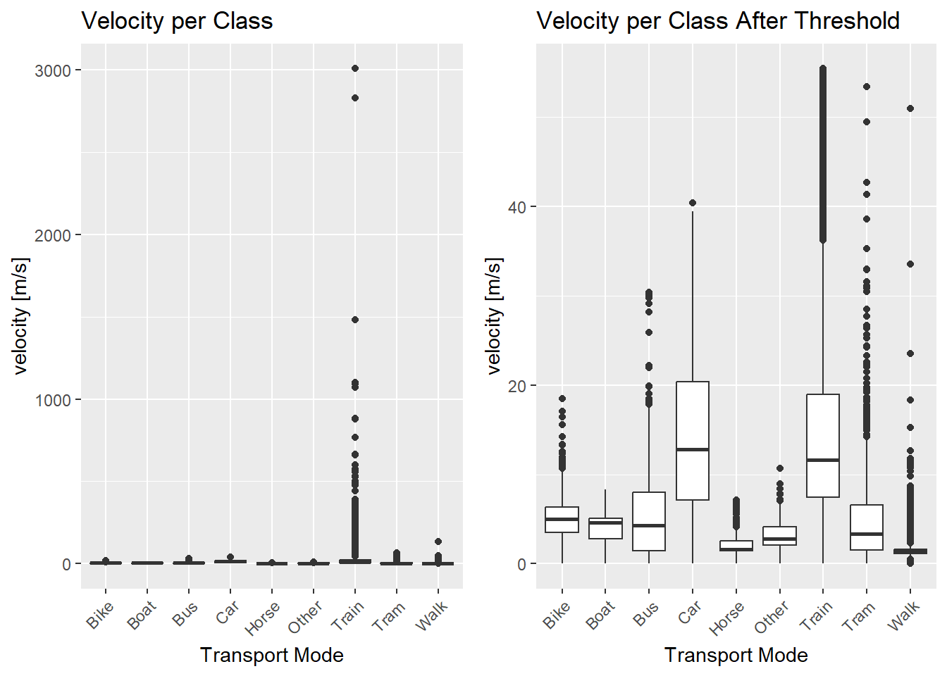
3.7.1 Velocity

The velocity attribute shows some outliers for the train class and walking class. The threshold for maximum velocity is set to 55.55 m/s (200km/h ), as no transport mode in our analysis is expected to exceed such velocity. One exception are airplanes, but with only very few data points there is no benefit in including higher velocities. After setting the threshold some obvious outliers remain for the walking class. Reasons for such outliers in the calculated velocity could be:

• Wrong Classification, even though the data is verified.

• GPS inaccuracies, where the GPS point location is “jumping” creating very inaccurate, zigzagging tracking data.

Code

boxplot_velocity <- ggplot(working_dataset, aes(x = transport_mode, y = velocity)) +
  geom_boxplot() +
  theme(axis.text.x = element_text(angle = 45, hjust = 1)) +
  ylab("velocity [m/s]") + xlab("Transport Mode") +
  ggtitle("Velocity per Class")

# Set threshold for parameters
working_dataset <- working_dataset[working_dataset$velocity < 55.55,]

boxplot_velocity_after <- ggplot(working_dataset, aes(x = transport_mode, y = velocity)) +
  geom_boxplot() +
  theme(axis.text.x = element_text(angle = 45, hjust = 1)) +
  ylab("velocity [m/s]") + xlab("Transport Mode") +
  ggtitle("Velocity per Class After Threshold")

# Display the plots side by side
grid.arrange(boxplot_velocity, boxplot_velocity_after, nrow = 1)

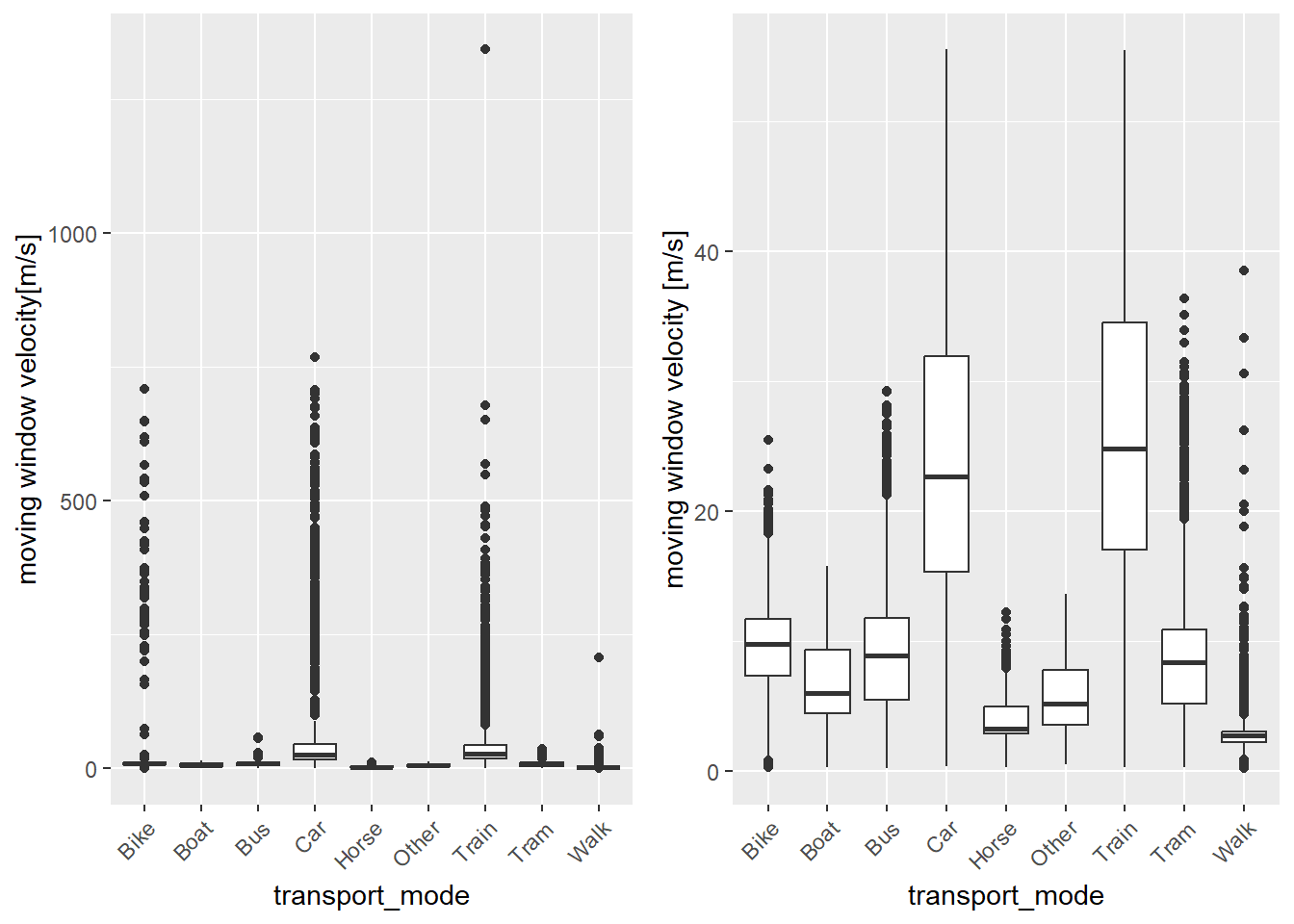
3.7.2 Moving Window Velocity

The moving window velocity shows less extreme outliers. The number of outliers can be reduced further by removing setting the trheshold to 55.5m/s (200km/h). After applying the threshold classes with similar average velocities can be identified. This might already be an indicator for classes which are difficult to distinguish using classification methods.

Code

boxplot_velocity_mean <- ggplot(working_dataset, aes(x = transport_mode, y = velocity_mean)) +
  geom_boxplot() +
  theme(axis.text.x = element_text(angle = 45, hjust = 1)) +
  ylab("moving window velocity[m/s]")

# Set threshold for parameters
working_dataset <- working_dataset[working_dataset$velocity_mean < 55.55,]

boxplot_velocity_mean_after <- ggplot(working_dataset, aes(x = transport_mode, y = velocity_mean)) +
  geom_boxplot() +
  theme(axis.text.x = element_text(angle = 45, hjust = 1)) +
  ylab("moving window velocity [m/s]")

# Display the plots side by side
grid.arrange(boxplot_velocity_mean, boxplot_velocity_mean_after, nrow = 1)

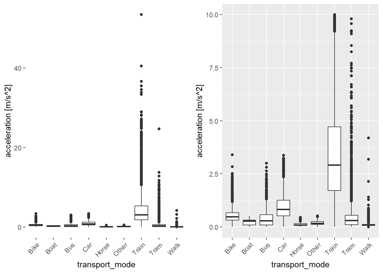
3.7.3 Acceleration

The acceleration threshold is set to 10m/s^2, as for this classification is considered to be the maximum possible acceleration for all classes. The distribution of the classes is similar to the velocities. In the parameter correlation analysis strong correlation between velocity and acceleration was found.

Code

boxplot_acceleration <- ggplot(working_dataset, aes(x = transport_mode, y = acceleration)) +
  geom_boxplot() +
  theme(axis.text.x = element_text(angle = 45, hjust = 1)) +
  ylab("acceleration [m/s^2]")

# Set threshold for parameters
working_dataset <- working_dataset[working_dataset$acceleration < 10,]

boxplot_acceleration_after <- ggplot(working_dataset, aes(x = transport_mode, y = acceleration)) +
  geom_boxplot() +
  theme(axis.text.x = element_text(angle = 45, hjust = 1)) +
  ylab("acceleration [m/s^2]")

# Display the plots side by side
grid.arrange(boxplot_acceleration, boxplot_acceleration_after, nrow = 1)

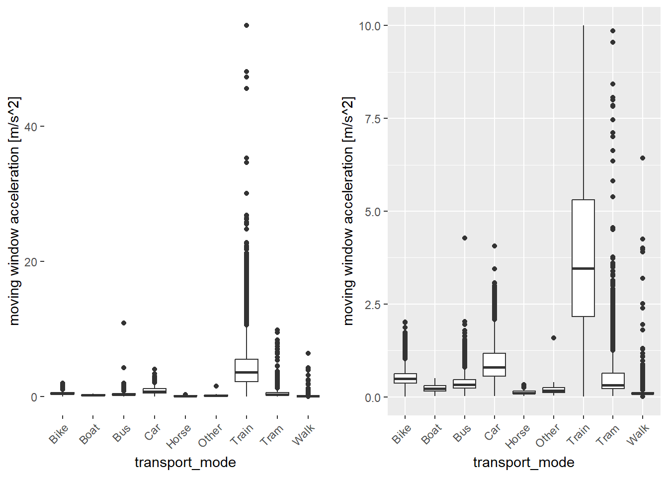
3.7.4 Moving Window Acceleration

The acceleration threshold is set to \(10m/s^2\), as for the single point acceleration values.

Code

boxplot_acceleration_mean <- ggplot(working_dataset, aes(x = transport_mode, y = acceleration_mean)) +
  geom_boxplot() +
  theme(axis.text.x = element_text(angle = 45, hjust = 1)) +
  ylab("moving window acceleration [m/s^2]")

# Set threshold for parameters
working_dataset <- working_dataset[working_dataset$acceleration_mean < 10,]

boxplot_acceleration_mean_after <- ggplot(working_dataset, aes(x = transport_mode, y = acceleration_mean)) +
  geom_boxplot() +
  theme(axis.text.x = element_text(angle = 45, hjust = 1)) +
  ylab("moving window acceleration [m/s^2]")

# Display the plots side by side
grid.arrange(boxplot_acceleration_mean, boxplot_acceleration_mean_after, nrow = 1)

3.8 Under Sampling

The data set is strongly imbalanced. To improve model accuracy under sampling was used to balance the classes. 500 samples per class are desired. The classes “boat” and “other” do not have sufficient points. The sample size is not further decreased, so enough data is provided to train the and test the computed models.

Code

set.seed(100)
# Create copy for later use
working_dataset_full <- working_dataset

# Set the maximum number of entries per class
max_entries <- 500

# Perform under sampling
working_dataset <- working_dataset |>
  group_by(transport_mode) |>
  sample_n(min(n(), max_entries)) |>
  ungroup()

# Check the resulting undersampled DataFrame
table(working_dataset$transport_mode)

 Bike  Boat   Bus   Car Horse Other Train  Tram  Walk 
  500   352   500   500   500   395   500   500   500 

Code

#Drop unwanted/Geom Columns
working_dataset <- working_dataset[,-c(1,3:5)]
working_dataset <- st_drop_geometry(working_dataset)

3.9 Classification

To classify the data a Support Vector Machine (SVM) is applied. A linear SVM, radial SVM and polynomial SVM are tested. A single-train-test split model and a 10 fold cross validation with 3 repeats was applied. The cross validation improves model robustness compared to the single train-test split and reduces bias resulting in a more representative evaluation of the model performance. The tuning sequences are replaced by the best found hyper parameters for each model, to save computation time.

The models are evaluated with the confusion matrix, the overall accuracy, recall, precision, and F1-Score. A confusion matrix is a table that summarizes the performance of a classification model by showing the counts of true positive, true negative, false positive, and false negative predictions. Precision measures the proportion of correctly predicted positive instances out of the total instances predicted as positive. Recall measures the proportion of correctly predicted positive instances out of the total actual positive instances. The F1-score combines precision and recall into a single metric. It provides a balance between precision and recall and is useful when both false positives and false negatives are important.

Code

# Define Control for 10-fold CV
fitControl <- trainControl(## 10-fold CV
                           method = "repeatedcv",
                           number = 10,
                           repeats = 3)

A training and a test data set is created. The training data set contains 80% of the data points and the test set contains 20% of the data points.

Code

set.seed(100)
# Convert to Factor
working_dataset$transport_mode <- as.factor(working_dataset$transport_mode)

# Create Training and Test Data Set
TrainingIndex <- createDataPartition(working_dataset$transport_mode, p = 0.8, list = F)
TrainingSet <- working_dataset[TrainingIndex,]
TestingSet <- working_dataset[-TrainingIndex,]

3.9.1 Liner SVM

A linear support vector machine is tested and the performance evaluated. Different hyper parameter settings were tested to find the best model. For the linear SVM the best fit found is for C = 3 achieving an overall accuracy of 77.87%. Precision, recall and F1-score vary for the classes but average around 78-79%.

Code

# Set seed for reproducibility
set.seed(100)

# Perform Linear SVM
model.svmL <- train(transport_mode ~ ., 
               data = TrainingSet,
               method = "svmLinear",
               na.action = na.omit,
               preprocess = c("scale", "center"),
               trControl = trainControl(method = "none"),
               tuneGrid = data.frame(C = 3),
               )

# Perform Linear SVM with 10-fold Cross Validation (Reduce Length for shorter computation time)
model.svmL.cv <- train(transport_mode ~ ., 
               data = TrainingSet,
               method = "svmLinear",
               na.action = na.omit,
               preprocess = c("sclae","center"),
               trControl = fitControl,
               tuneGrid = expand.grid(C = seq(3, 6, length = 4) # Find best Fit Model
               ))

# Show Best Tune
#print(model.svmL.cv$bestTune)

# Make Predictions
model.svmL.training <- predict(model.svmL, TrainingSet)
model.svmL.testing <- predict(model.svmL, TestingSet)
model.svmL.cv.training <- predict(model.svmL.cv, TrainingSet)
model.svmL.cv.testing <- predict(model.svmL.cv, TrainingSet)

# Model Performance
model.svmL.training.confusion <- confusionMatrix(model.svmL.training, as.factor(TrainingSet$transport_mode))
model.svmL.testing.confusion <- confusionMatrix(model.svmL.testing, as.factor(TestingSet$transport_mode))
model.svmL.cv.training.confusion <- confusionMatrix(model.svmL.cv.training, as.factor(TrainingSet$transport_mode))
(model.svmL.cv.testing.confusion <- confusionMatrix(model.svmL.cv.testing, as.factor(TrainingSet$transport_mode))) # Print test run with CV

Confusion Matrix and Statistics

          Reference
Prediction Bike Boat Bus Car Horse Other Train Tram Walk
     Bike   263    0  60  30     1    17     4    8    2
     Boat     0  282   0   0     0     0     0    0    0
     Bus     36    0 210  10     0    22     4    6   25
     Car      6    0  26 334     1    13     1    0    0
     Horse   11    0   6   7   390    13     0    0   93
     Other    5    0  11   3     1   185     0    2    8
     Train    2    0   1   1     0     0   388    0    1
     Tram    66    0  67   9     0    40     0  362   39
     Walk    11    0  19   6     7    26     3   22  232

Overall Statistics
                                          
               Accuracy : 0.7787          
                 95% CI : (0.7644, 0.7926)
    No Information Rate : 0.1177          
    P-Value [Acc > NIR] : < 2.2e-16       
                                          
                  Kappa : 0.7504          
                                          
 Mcnemar's Test P-Value : NA              

Statistics by Class:

                     Class: Bike Class: Boat Class: Bus Class: Car Class: Horse
Sensitivity               0.6575     1.00000    0.52500    0.83500       0.9750
Specificity               0.9593     1.00000    0.96564    0.98432       0.9566
Pos Pred Value            0.6831     1.00000    0.67093    0.87664       0.7500
Neg Pred Value            0.9545     1.00000    0.93841    0.97812       0.9965
Prevalence                0.1177     0.08299    0.11772    0.11772       0.1177
Detection Rate            0.0774     0.08299    0.06180    0.09829       0.1148
Detection Prevalence      0.1133     0.08299    0.09211    0.11212       0.1530
Balanced Accuracy         0.8084     1.00000    0.74532    0.90966       0.9658
                     Class: Other Class: Train Class: Tram Class: Walk
Sensitivity               0.58544       0.9700      0.9050     0.58000
Specificity               0.99027       0.9983      0.9263     0.96865
Pos Pred Value            0.86047       0.9873      0.6209     0.71166
Neg Pred Value            0.95884       0.9960      0.9865     0.94531
Prevalence                0.09300       0.1177      0.1177     0.11772
Detection Rate            0.05444       0.1142      0.1065     0.06828
Detection Prevalence      0.06327       0.1157      0.1716     0.09594
Balanced Accuracy         0.78785       0.9842      0.9156     0.77432

Code

# Precision for each class
cat("\nPrecision for each class:\n")

Precision for each class:

Code

(precision_svmL <- model.svmL.cv.testing.confusion$byClass[, "Precision"])

 Class: Bike  Class: Boat   Class: Bus   Class: Car Class: Horse Class: Other 
   0.6831169    1.0000000    0.6709265    0.8766404    0.7500000    0.8604651 
Class: Train  Class: Tram  Class: Walk 
   0.9872774    0.6209262    0.7116564 

Code

cat("\nAverage Precision:\n")

Average Precision:

Code

(precision_svmL <- mean(model.svmL.cv.testing.confusion$byClass[, "Precision"]))

[1] 0.7956677

Code

# Recall for each class
cat("\nRecall for each class:\n")

Recall for each class:

Code

(recall_svmL<- model.svmL.cv.testing.confusion$byClass[, "Recall"])

 Class: Bike  Class: Boat   Class: Bus   Class: Car Class: Horse Class: Other 
    0.657500     1.000000     0.525000     0.835000     0.975000     0.585443 
Class: Train  Class: Tram  Class: Walk 
    0.970000     0.905000     0.580000 

Code

cat("\nAverage Recall:\n")

Average Recall:

Code

(recall_svmL <- mean(model.svmL.cv.testing.confusion$byClass[, "Recall"]))

[1] 0.7814381

Code

# F1-Score for each class
cat("\nF1-Score for each class:\n")

F1-Score for each class:

Code

(f1_score_svmL <- model.svmL.cv.testing.confusion$byClass[, "F1"])

 Class: Bike  Class: Boat   Class: Bus   Class: Car Class: Horse Class: Other 
   0.6700637    1.0000000    0.5890603    0.8553137    0.8478261    0.6967985 
Class: Train  Class: Tram  Class: Walk 
   0.9785624    0.7365209    0.6391185 

Code

cat("\nAverage F1-Score:\n")

Average F1-Score:

Code

(f1_score_svmL <- mean(model.svmL.cv.testing.confusion$byClass[, "F1"]))

[1] 0.7792516

Code

# Save the models
saveRDS(model.svmL, "models/model_svmL.rds")
saveRDS(model.svmL.cv, "models/model_svmL_cv.rds")

3.9.2 Radial Support Vector Machine

The radial SVM performs slightly better than the linear SVM with an overall accuracy of 79.27% and similar recall, precision and f1-scores. This model however performs better, since the applied metrics vary less between classes.

Code

# Set seed for reproduceability
set.seed(108)

# Build Training Model
model.svmRadial <- train(transport_mode ~ .,
                         data = TrainingSet,
                         method = "svmRadial",
                         na.action = na.omit,
                         preprocess = c("scale", "center"),
                         trControl = trainControl(method = "none"),
                         tuneGrid = expand.grid(sigma = 0.8683492, C = 5)
)             

# Build CV Model (long processing!!!)
TrainingSet$transport_mode <- as.character(TrainingSet$transport_mode)
model.svmRadial.cv <- train(transport_mode ~ .,
                            data = TrainingSet,
                            method = "svmRadial",
                            na.action = na.omit,
                            preprocess = c("scale", "center"),
                            trControl = fitControl,
                            tuneGrid = expand.grid(sigma = 0.8683492, C = 5)
)
               
(model.svmRadial.cv$bestTune)

      sigma C
1 0.8683492 5

Code

# Make Predictions
model.svmRadial.training <- predict(model.svmRadial, TrainingSet)
model.svmRadial.testing <- predict(model.svmRadial, TestingSet)

# Make Predictions from Cross Validation model
model.svmRadial.cv.training <- predict(model.svmRadial.cv, TrainingSet)
model.svmRadial.cv.testing <- predict(model.svmRadial.cv, TestingSet)

# Model Performance
model.svmRadial.training.confusion <- confusionMatrix(model.svmRadial.training, as.factor(TrainingSet$transport_mode))
model.svmRadial.testing.confusion <- confusionMatrix(model.svmRadial.testing, as.factor(TestingSet$transport_mode))
model.svmRadial.cv.confusion <- confusionMatrix(model.svmRadial.cv.training, as.factor(TrainingSet$transport_mode))
(model.svmRadial.cv.testing.confusion <- confusionMatrix(model.svmRadial.cv.testing, as.factor(TestingSet$transport_mode))) # Print test run with CV

Confusion Matrix and Statistics

          Reference
Prediction Bike Boat Bus Car Horse Other Train Tram Walk
     Bike    71    0  10   4     1     6     1    1    1
     Boat     0   66   0   0     0     0     0    0    0
     Bus     11    0  55   4     0     3     0    2    7
     Car      2    0   6  85     0     1     0    1    0
     Horse    3    0   1   1    97     1     0    0   27
     Other    3    0   1   1     0    56     0    1   12
     Train    1    4   7   5     0     3    99    4    7
     Tram     7    0  16   0     0     6     0   86    9
     Walk     2    0   4   0     2     3     0    5   37

Overall Statistics
                                         
               Accuracy : 0.768          
                 95% CI : (0.7381, 0.796)
    No Information Rate : 0.1178         
    P-Value [Acc > NIR] : < 2.2e-16      
                                         
                  Kappa : 0.7384         
                                         
 Mcnemar's Test P-Value : NA             

Statistics by Class:

                     Class: Bike Class: Boat Class: Bus Class: Car Class: Horse
Sensitivity              0.71000     0.94286    0.55000     0.8500       0.9700
Specificity              0.96796     1.00000    0.96395     0.9866       0.9559
Pos Pred Value           0.74737     1.00000    0.67073     0.8947       0.7462
Neg Pred Value           0.96154     0.99489    0.94133     0.9801       0.9958
Prevalence               0.11779     0.08245    0.11779     0.1178       0.1178
Detection Rate           0.08363     0.07774    0.06478     0.1001       0.1143
Detection Prevalence     0.11190     0.07774    0.09658     0.1119       0.1531
Balanced Accuracy        0.83898     0.97143    0.75698     0.9183       0.9630
                     Class: Other Class: Train Class: Tram Class: Walk
Sensitivity               0.70886       0.9900      0.8600     0.37000
Specificity               0.97662       0.9586      0.9493     0.97864
Pos Pred Value            0.75676       0.7615      0.6935     0.69811
Neg Pred Value            0.97032       0.9986      0.9807     0.92085
Prevalence                0.09305       0.1178      0.1178     0.11779
Detection Rate            0.06596       0.1166      0.1013     0.04358
Detection Prevalence      0.08716       0.1531      0.1461     0.06243
Balanced Accuracy         0.84274       0.9743      0.9046     0.67432

Code

# Precision for each class
cat("\nPrecision for each class:\n")

Precision for each class:

Code

(precision_svmRadial <- model.svmRadial.cv.testing.confusion$byClass[, "Precision"])

 Class: Bike  Class: Boat   Class: Bus   Class: Car Class: Horse Class: Other 
   0.7473684    1.0000000    0.6707317    0.8947368    0.7461538    0.7567568 
Class: Train  Class: Tram  Class: Walk 
   0.7615385    0.6935484    0.6981132 

Code

cat("\nAverage Precision:\n")

Average Precision:

Code

(precision_svmRadial_avg <- mean(model.svmRadial.cv.testing.confusion$byClass[, "Precision"]))

[1] 0.7743275

Code

# Recall for each class
cat("\nRecall for each class:\n")

Recall for each class:

Code

(recall_svmRadial<- model.svmRadial.cv.testing.confusion$byClass[, "Recall"])

 Class: Bike  Class: Boat   Class: Bus   Class: Car Class: Horse Class: Other 
   0.7100000    0.9428571    0.5500000    0.8500000    0.9700000    0.7088608 
Class: Train  Class: Tram  Class: Walk 
   0.9900000    0.8600000    0.3700000 

Code

cat("\nAverage Recall:\n")

Average Recall:

Code

(recall_svmRadial_avg <- mean(model.svmRadial.cv.testing.confusion$byClass[, "Recall"]))

[1] 0.7724131

Code

# F1-Score for each class
cat("\nF1-Score for each class:\n")

F1-Score for each class:

Code

(f1_score_svmRadial <- model.svmRadial.cv.testing.confusion$byClass[, "F1"])

 Class: Bike  Class: Boat   Class: Bus   Class: Car Class: Horse Class: Other 
   0.7282051    0.9705882    0.6043956    0.8717949    0.8434783    0.7320261 
Class: Train  Class: Tram  Class: Walk 
   0.8608696    0.7678571    0.4836601 

Code

cat("\nAverage F1-Score:\n")

Average F1-Score:

Code

(f1_score_svmRadial_avg <- mean(model.svmRadial.cv.testing.confusion$byClass[, "F1"]))

[1] 0.7625417

Code

# Save the models
saveRDS(model.svmRadial, "models/model_svmRadial.rds")
saveRDS(model.svmRadial.cv, "models/model_svmRadial_cv.rds")

3.9.3 Polynomial SVM

Out of all tested models the polynomial SVM achieved the highest overall accuracy with 79.15% and the best performance for recall, precision and F1-score. The by class performance is significantly better compared to the other models. The Cohen’s Kappa value lies at 0.76 indicating high agreement between the predictions and ground truth labels. The p-value indicates that the accuracy of the polynomial SVM model is significantly better than the no information rate.

Code

set.seed(100)

# Build Training Model
model.svmPoly <- train(transport_mode ~ ., 
               data = TrainingSet,
               method = "svmPoly",
               na.action = na.omit,
               preprocess = c("sclae","center"),
               trControl = trainControl(method = "none"),
               tuneGrid = data.frame(degree = 3, scale = 0.1, C = 4)
               )
               

# Build CV Model (long processing)
TrainingSet$transport_mode <- as.character(TrainingSet$transport_mode)
model.svmPoly.cv <- train(transport_mode ~ ., 
               data = TrainingSet,
               method = "svmPoly",
               na.action = na.omit,
               preprocess = c("sclae","center"),
               trControl = fitControl,
               tuneGrid = data.frame(degree = 3, scale = 0.1, C = 4) # Fit Model) 
               )
                
               
(model.svmPoly.cv$bestTune)

  degree scale C
1      3   0.1 4

Code

# Make Predictions
model.svmPoly.training <- predict(model.svmPoly, TrainingSet)
model.svmPoly.testing <- predict(model.svmPoly, TestingSet)

# Make Predictions from Cross Validation model
model.svmPoly.cv.training <- predict(model.svmPoly.cv, TrainingSet)
model.svmPoly.cv.testing <- predict(model.svmPoly.cv, TestingSet)

# Model Performance
model.svmPoly.training.confusion <- confusionMatrix(model.svmPoly.training, as.factor(TrainingSet$transport_mode))
model.svmPoly.testing.confusion <- confusionMatrix(model.svmPoly.testing, as.factor(TestingSet$transport_mode))
model.svmPoly.cv.confusion <- confusionMatrix(model.svmPoly.cv.training, as.factor(TrainingSet$transport_mode))
(model.svmPoly.cv.testing.confusion <- confusionMatrix(model.svmPoly.cv.testing, as.factor(TestingSet$transport_mode))) # Print test run with CV

Confusion Matrix and Statistics

          Reference
Prediction Bike Boat Bus Car Horse Other Train Tram Walk
     Bike    77    0  16   4     0     2     1    3    0
     Boat     0   70   0   0     0     0     0    0    0
     Bus      5    0  48   5     0     3     2    3    4
     Car      3    0  11  86     0     2     2    0    1
     Horse    2    0   1   2    97     2     0    0   27
     Other    4    0   4   1     1    60     0    0    8
     Train    0    0   2   1     0     0    95    1    1
     Tram     9    0  13   0     0     5     0   89   14
     Walk     0    0   5   1     2     5     0    4   45

Overall Statistics
                                          
               Accuracy : 0.7856          
                 95% CI : (0.7565, 0.8128)
    No Information Rate : 0.1178          
    P-Value [Acc > NIR] : < 2.2e-16       
                                          
                  Kappa : 0.7584          
                                          
 Mcnemar's Test P-Value : NA              

Statistics by Class:

                     Class: Bike Class: Boat Class: Bus Class: Car Class: Horse
Sensitivity              0.77000     1.00000    0.48000     0.8600       0.9700
Specificity              0.96529     1.00000    0.97063     0.9746       0.9546
Pos Pred Value           0.74757     1.00000    0.68571     0.8190       0.7405
Neg Pred Value           0.96917     1.00000    0.93325     0.9812       0.9958
Prevalence               0.11779     0.08245    0.11779     0.1178       0.1178
Detection Rate           0.09069     0.08245    0.05654     0.1013       0.1143
Detection Prevalence     0.12132     0.08245    0.08245     0.1237       0.1543
Balanced Accuracy        0.86764     1.00000    0.72531     0.9173       0.9623
                     Class: Other Class: Train Class: Tram Class: Walk
Sensitivity               0.75949       0.9500      0.8900     0.45000
Specificity               0.97662       0.9933      0.9453     0.97730
Pos Pred Value            0.76923       0.9500      0.6846     0.72581
Neg Pred Value            0.97536       0.9933      0.9847     0.93011
Prevalence                0.09305       0.1178      0.1178     0.11779
Detection Rate            0.07067       0.1119      0.1048     0.05300
Detection Prevalence      0.09187       0.1178      0.1531     0.07303
Balanced Accuracy         0.86806       0.9717      0.9176     0.71365

Code

# Precision for each class
cat("\nPrecision for each class:\n")

Precision for each class:

Code

(precision_svmPoly <- model.svmPoly.cv.testing.confusion$byClass[, "Precision"])

 Class: Bike  Class: Boat   Class: Bus   Class: Car Class: Horse Class: Other 
   0.7475728    1.0000000    0.6857143    0.8190476    0.7404580    0.7692308 
Class: Train  Class: Tram  Class: Walk 
   0.9500000    0.6846154    0.7258065 

Code

cat("\nAverage Precision:\n")

Average Precision:

Code

(precision_svmPoly_avg <- mean(model.svmPoly.cv.testing.confusion$byClass[, "Precision"]))

[1] 0.7913828

Code

# Recall for each class
cat("\nRecall for each class:\n")

Recall for each class:

Code

(recall_svmPoly <- model.svmPoly.cv.testing.confusion$byClass[, "Recall"])

 Class: Bike  Class: Boat   Class: Bus   Class: Car Class: Horse Class: Other 
   0.7700000    1.0000000    0.4800000    0.8600000    0.9700000    0.7594937 
Class: Train  Class: Tram  Class: Walk 
   0.9500000    0.8900000    0.4500000 

Code

cat("\nAverage Recall:\n")

Average Recall:

Code

(recall_svmPoly_avg <- mean(model.svmPoly.cv.testing.confusion$byClass[, "Recall"]))

[1] 0.792166

Code

# F1-Score for each class
cat("\nF1-Score for each class:\n")

F1-Score for each class:

Code

(f1_score_svmPoly <- model.svmPoly.cv.testing.confusion$byClass[, "F1"])

 Class: Bike  Class: Boat   Class: Bus   Class: Car Class: Horse Class: Other 
   0.7586207    1.0000000    0.5647059    0.8390244    0.8398268    0.7643312 
Class: Train  Class: Tram  Class: Walk 
   0.9500000    0.7739130    0.5555556 

Code

cat("\nAverage F1-Score:\n")

Average F1-Score:

Code

(f1_score_svmPoly_avg <- mean(model.svmPoly.cv.testing.confusion$byClass[, "F1"]))

[1] 0.7828864

Code

# Save the models
saveRDS(model.svmPoly, "models/model_svmPoly.rds")
saveRDS(model.svmPoly.cv, "models/model_svmPoly_cv.rds")

Since the polynomial SVM showed the best performance, this model is used to predict the transport mode on the full data set, containing 40’525 data points after preprocessing and threshold filtering. The achieved overall accuracy is 81.65% with the 95% confidence interval of [81.27%, 82.03%]. The full data set is very imbalanced, nevertheless the unweighted averaged F1-score lies at 75%

Code

# Set seed for reproducibility
set.seed(100)

# Run Model on full data set
model.final <- predict(model.svmPoly.cv, working_dataset_full)

# Create final data frame
working_dataset_result <- data.frame(working_dataset_full, model.final) 

# Confusion Matrix for new results
conf_matrix <- confusionMatrix(as.factor(working_dataset_result$transport_mode), as.factor(working_dataset_result$model.final))
cat("Confusion Matrix:\n")

Confusion Matrix:

Code

conf_matrix

Confusion Matrix and Statistics

          Reference
Prediction  Bike  Boat   Bus   Car Horse Other Train  Tram  Walk
     Bike   1520     0    79    24    40    70     2    91    27
     Boat      0   352     0     0     0     0     0     0     0
     Bus     494     0  2015   286    45   146    18   533   199
     Car     343     0   228  4408   125   146    26    26    49
     Horse    15     0     2     6  3613    18     0     0    63
     Other     4     0     4     5    14   320     0    28    20
     Train   137     0    67   110     1     4 12379    69    17
     Tram    165     0   106    22     0    35    48  3945   177
     Walk    140     0   220    34  1866   447    19   633  4483

Overall Statistics
                                          
               Accuracy : 0.8151          
                 95% CI : (0.8113, 0.8189)
    No Information Rate : 0.3082          
    P-Value [Acc > NIR] : < 2.2e-16       
                                          
                  Kappa : 0.7761          
                                          
 Mcnemar's Test P-Value : NA              

Statistics by Class:

                     Class: Bike Class: Boat Class: Bus Class: Car Class: Horse
Sensitivity              0.53939    1.000000    0.74054     0.9005      0.63342
Specificity              0.99117    1.000000    0.95448     0.9735      0.99701
Pos Pred Value           0.82029    1.000000    0.53935     0.8238      0.97202
Neg Pred Value           0.96644    1.000000    0.98081     0.9862      0.94320
Prevalence               0.06953    0.008685    0.06714     0.1208      0.14074
Detection Rate           0.03750    0.008685    0.04972     0.1088      0.08915
Detection Prevalence     0.04572    0.008685    0.09218     0.1320      0.09171
Balanced Accuracy        0.76528    1.000000    0.84751     0.9370      0.81521
                     Class: Other Class: Train Class: Tram Class: Walk
Sensitivity              0.269815       0.9910     0.74085      0.8904
Specificity              0.998094       0.9856     0.98429      0.9054
Pos Pred Value           0.810127       0.9683     0.87706      0.5717
Neg Pred Value           0.978422       0.9959     0.96170      0.9831
Prevalence               0.029264       0.3082     0.13139      0.1242
Detection Rate           0.007896       0.3054     0.09734      0.1106
Detection Prevalence     0.009746       0.3154     0.11098      0.1935
Balanced Accuracy        0.633954       0.9883     0.86257      0.8979

Code

# Precision for each class
precision <- conf_matrix$byClass[, "Precision"]
cat("\nPrecision for each class:\n")

Precision for each class:

Code

precision

 Class: Bike  Class: Boat   Class: Bus   Class: Car Class: Horse Class: Other 
   0.8202914    1.0000000    0.5393469    0.8237713    0.9720204    0.8101266 
Class: Train  Class: Tram  Class: Walk 
   0.9683198    0.8770565    0.5716654 

Code

# Average Precision
avg_precision <- mean(conf_matrix$byClass[, "Precision"])
cat("\nAverage Precision:\n")

Average Precision:

Code

avg_precision

[1] 0.8202887

Code

# Recall for each class
recall <- conf_matrix$byClass[, "Recall"]
cat("\nRecall for each class:\n")

Recall for each class:

Code

recall

 Class: Bike  Class: Boat   Class: Bus   Class: Car Class: Horse Class: Other 
   0.5393896    1.0000000    0.7405366    0.9005107    0.6334151    0.2698145 
Class: Train  Class: Tram  Class: Walk 
   0.9909542    0.7408451    0.8903674 

Code

# Average Recall
avg_recall <- mean(conf_matrix$byClass[, "Recall"])
cat("\nAverage Recall:\n")

Average Recall:

Code

avg_recall

[1] 0.7450926

Code

# F1-Score for each class
f1_score <- conf_matrix$byClass[, "F1"]
cat("\nF1-Score for each class:\n")

F1-Score for each class:

Code

f1_score

 Class: Bike  Class: Boat   Class: Bus   Class: Car Class: Horse Class: Other 
   0.6508242    1.0000000    0.6241289    0.8604333    0.7670099    0.4048071 
Class: Train  Class: Tram  Class: Walk 
   0.9795063    0.8032169    0.6962802 

Code

# Average F1-Score
avg_f1_score <- mean(conf_matrix$byClass[, "F1"])
cat("\nAverage F1-Score:\n")

Average F1-Score:

Code

avg_f1_score

[1] 0.754023

Code

# Save working_dataset_result as a CSV file
write.csv(working_dataset_result, "data/working_dataset_result.csv", row.names = FALSE)

The resulting class distribution shows that the model predicts too many points as train. This boosts the models performance, since the train class is strongly over represented in this data set. A significant number of false classifications etween the transport modes Car, Bus, Bike and Tram was expected, since key parameters such as velocity and acceleration lie in similar ranges and are difficult to distinguish by the model.

Code

# Show class distribution
final_classes <- ggplot(working_dataset_full) + 
  geom_bar(aes(x = model.final)) +
  theme(axis.text.x = element_text(angle = 45, hjust = 1)) +
  geom_hline(yintercept = 500, colour = "red", linetype = "dashed") +
  ylim(c(0,14000)) + xlab("Transport Mode")

classes <- ggplot(working_dataset_result) + 
  geom_bar(aes(x = transport_mode)) +
  theme(axis.text.x = element_text(angle = 45, hjust = 1)) +
  geom_hline(yintercept = 500, colour = "red", linetype = "dashed") +
  ylim(c(0,14000)) + xlab("Transport Mode")

grid.arrange(classes, final_classes, nrow = 1)

Code

table(working_dataset_result$transport_mode)

 Bike  Boat   Bus   Car Horse Other Train  Tram  Walk 
 1853   352  3736  5351  3717   395 12784  4498  7842 

Code

table(working_dataset_result$model.final)

 Bike  Boat   Bus   Car Horse Other Train  Tram  Walk 
 2818   352  2721  4895  5704  1186 12492  5325  5035 

3.10 Post Processing

To boost the model performance some simple post processing is applied. A moving window function is used to find misclassified points within segments. This function searches within x neighbors of a point and if a given percentage of these points belong to one class the point is reclassified as the majority of its neighboring points. This process can be applied iteratively.

For this data set a window size of 1, a threshold percentage of 75% and 3 iterations results in a smoothing of the results, but not necessarily a gain in model accuracy. After postprocessing an increase of 3-4% overall accuracy was found.

Code

# Run a loop to identify outlier points in classification. If prevous and following x points are identical, 
# but the middle one is different it is changed


# Define the number of previous and following points to consider
# x: Number of points to be looked at surrounding current value in each direction (x*2 neighbours considered)
# threshold_percentage: number of points which have to be equal so the current value gets changed
# i: number of iterations

single_point_correction <- function(df, x, threshold_percentage, iterations) {
  
  # Track the number of points changed
  changed_count <- 0  
  
  for (iter in 1:iterations) {
    for (i in (x + 1):(nrow(df) - x)) {
      current_value <- df$model.final[i]
      
      # Find x-Previous & x-Following Values around point i
      previous_values <- df$model.final[(i - x):(i - 1)]
      following_values <- df$model.final[(i + 1):(i + x)]
      
      # Calculate the number of occurrences for each class in the surrounding points
      class_counts <- table(c(previous_values, following_values))
      
      # Find the class that occurs most frequently
      most_frequent_class <- names(class_counts)[which.max(class_counts)]
      
      # Check if the most frequent class exceeds the threshold count
      if (class_counts[most_frequent_class] > threshold_percentage * length(c(previous_values, following_values))) {
        df$model.final[i] <- most_frequent_class
        changed_count <- changed_count + 1
      }
    }
  message("Metrics after each iteration:")
  conf_matrix_func <- confusionMatrix(as.factor(df$transport_mode), as.factor(df$model.final))
  # Precision for each class
  cat("\n Mean Precision\n")
  print(precision_func <- mean(conf_matrix_func$byClass[, "Precision"]))
  # Recall for each class
  cat("\n Mean Recall\n")
  print(recall_func <- mean(conf_matrix_func$byClass[, "Recall"]))
  # F1-Score for each class
  cat("\n Mean F1-Score\n")
  print(f1_score_func <- mean(conf_matrix_func$byClass[, "F1"]))
  
  }
  

  message("Number of times the condition is true and values are updated:", changed_count)
  

  return(df)
}

working_dataset_result_copy <- working_dataset_result
working_dataset_result <- single_point_correction(working_dataset_result, 10, 0.75, 3)

 Mean Precision
[1] 0.8486992

 Mean Recall
[1] 0.7729815

 Mean F1-Score
[1] 0.7830847

 Mean Precision
[1] 0.8491123

 Mean Recall
[1] 0.7735217

 Mean F1-Score
[1] 0.783549

 Mean Precision
[1] 0.8491773

 Mean Recall
[1] 0.7735824

 Mean F1-Score
[1] 0.7835973

Code

# Confusion Matrix for new results
conf_matrix_2 <- confusionMatrix(as.factor(working_dataset_result$transport_mode), as.factor(working_dataset_result$model.final))
cat("Confusion Matrix:\n")

Confusion Matrix:

Code

conf_matrix_2

Confusion Matrix and Statistics

          Reference
Prediction  Bike  Boat   Bus   Car Horse Other Train  Tram  Walk
     Bike   1669     0    19    12    38    57     0    48    10
     Boat      0   352     0     0     0     0     0     0     0
     Bus     485     0  2116   295    43   133    15   457   192
     Car     346     0   174  4535   101   106    17    23    49
     Horse     0     0     0     3  3702     1     0     0    11
     Other     3     0     3     5    14   338     0    21    11
     Train    96     0    47    82     1     4 12497    41    16
     Tram     87     0    57    22     0    18    20  4145   149
     Walk    113     0   200    35  1977   337    17   636  4527

Overall Statistics
                                          
               Accuracy : 0.836           
                 95% CI : (0.8323, 0.8396)
    No Information Rate : 0.3101          
    P-Value [Acc > NIR] : < 2.2e-16       
                                          
                  Kappa : 0.8012          
                                          
 Mcnemar's Test P-Value : NA              

Statistics by Class:

                     Class: Bike Class: Boat Class: Bus Class: Car Class: Horse
Sensitivity              0.59628    1.000000    0.80887     0.9090      0.63002
Specificity              0.99512    1.000000    0.95727     0.9770      0.99957
Pos Pred Value           0.90070    1.000000    0.56638     0.8475      0.99596
Neg Pred Value           0.97078    1.000000    0.98641     0.9871      0.94094
Prevalence               0.06906    0.008685    0.06455     0.1231      0.14499
Detection Rate           0.04118    0.008685    0.05221     0.1119      0.09134
Detection Prevalence     0.04572    0.008685    0.09218     0.1320      0.09171
Balanced Accuracy        0.79570    1.000000    0.88307     0.9430      0.81479
                     Class: Other Class: Train Class: Tram Class: Walk
Sensitivity              0.340040       0.9945      0.7717      0.9118
Specificity              0.998558       0.9897      0.9900      0.9068
Pos Pred Value           0.855696       0.9776      0.9215      0.5773
Neg Pred Value           0.983654       0.9975      0.9660      0.9866
Prevalence               0.024526       0.3101      0.1325      0.1225
Detection Rate           0.008340       0.3084      0.1023      0.1117
Detection Prevalence     0.009746       0.3154      0.1110      0.1935
Balanced Accuracy        0.669299       0.9921      0.8808      0.9093

Code

# Precision for each class
precision_2 <- conf_matrix_2$byClass[, "Precision"]
cat("\nPrecision for each class:\n")

Precision for each class:

Code

precision_2

 Class: Bike  Class: Boat   Class: Bus   Class: Car Class: Horse Class: Other 
   0.9007016    1.0000000    0.5663812    0.8475051    0.9959645    0.8556962 
Class: Train  Class: Tram  Class: Walk 
   0.9775501    0.9215207    0.5772762 

Code

# Average Precision
avg_precision_2 <- mean(conf_matrix_2$byClass[, "Precision"])
cat("\nAverage Precision:\n")

Average Precision:

Code

avg_precision_2

[1] 0.8491773

Code

# Recall for each class
recall_2 <- conf_matrix_2$byClass[, "Recall"]
cat("\nRecall for each class:\n")

Recall for each class:

Code

recall_2

 Class: Bike  Class: Boat   Class: Bus   Class: Car Class: Horse Class: Other 
   0.5962844    1.0000000    0.8088685    0.9089998    0.6300204    0.3400402 
Class: Train  Class: Tram  Class: Walk 
   0.9945090    0.7717371    0.9117825 

Code

# Average Recall
avg_recall_2 <- mean(conf_matrix_2$byClass[, "Recall"])
cat("\nAverage Recall:\n")

Average Recall:

Code

avg_recall_2

[1] 0.7735824

Code

# F1-Score for each class
f1_score_2 <- conf_matrix_2$byClass[, "F1"]
cat("\nF1-Score for each class:\n")

F1-Score for each class:

Code

f1_score_2

 Class: Bike  Class: Boat   Class: Bus   Class: Car Class: Horse Class: Other 
   0.7175408    1.0000000    0.6662469    0.8771760    0.7718128    0.4866811 
Class: Train  Class: Tram  Class: Walk 
   0.9859566    0.8400041    0.7069571 

Code

# Average F1-Score
avg_f1_score <- mean(conf_matrix_2$byClass[, "F1"])
cat("\nAverage F1-Score:\n")

Average F1-Score:

Code

avg_f1_score

[1] 0.7835973

Code

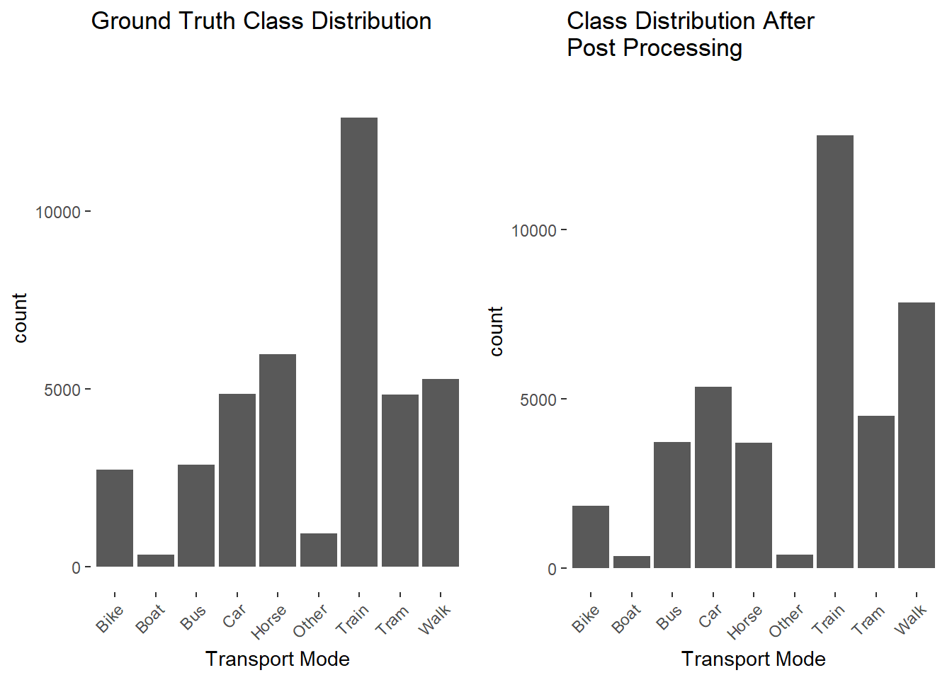
# Show class distribution
final_classes <- ggplot(working_dataset_result) + 
  geom_bar(aes(x = model.final)) +
  theme(axis.text.x = element_text(angle = 45, hjust = 1)) +
  ylim(c(0,14000)) +
  ggtitle("Ground Truth Class Distribution") +
  xlab("Transport Mode")

classes <- ggplot(working_dataset_result) + 
  geom_bar(aes(x = transport_mode)) +
  theme(axis.text.x = element_text(angle = 45, hjust = 1)) +
  ylim(c(0,14000)) +
  ggtitle("Class Distribution After \nPost Processing") +
  xlab("Transport Mode")


grid.arrange(final_classes,classes, nrow = 1)

Code

cat("Ground Truth\n")

Ground Truth

Code

table(working_dataset_result$transport_mode)

 Bike  Boat   Bus   Car Horse Other Train  Tram  Walk 
 1853   352  3736  5351  3717   395 12784  4498  7842 

Code

cat("\nClassification \n")

Classification 

Code

table(working_dataset_result$model.final)

 Bike  Boat   Bus   Car Horse Other Train  Tram  Walk 
 2799   352  2616  4989  5876   994 12566  5371  4965 

The below map allows the comparison between wrongly classified points and ground truth to explore where the model fails.

Code

visualisation <- working_dataset_result %>%
  st_as_sf(coords = c("longitude", "latitude"), crs = 4326) %>%
  select(transport_mode, datetime, model.final) 

visualisation <- visualisation[10000:15000,] 


visualisation$colorTrue <- c("#7FC97F", "#BEAED4", "#FDC086", "#FFFF99", "#386CB0", "#F0027F", "#BF5B17")[match(visualisation$transport_mode, c("Bike", "Bus", "Car", "Other", "Train", "Tram", "Walk"))]

visualisation$colorModel <- c("#7FC97F", "#BEAED4", "#FDC086", "#FFFF99", "#386CB0", "#F0027F", "#BF5B17")[match(visualisation$model.final, c("Bike", "Bus", "Car", "Other", "Train", "Tram", "Walk"))]

length(unique(visualisation$model.final))

[1] 7

Code

length(unique(visualisation$transport_mode))

[1] 7

Code

wrong_points <- visualisation %>%
  filter(model.final != transport_mode)

palTrue <- c("#7FC97F", "#BEAED4", "#FDC086", "#FFFF99", "#386CB0", "#F0027F", "#BF5B17")
palModel <- c("#7FC97F", "#BEAED4", "#FDC086", "#FFFF99", "#386CB0", "#F0027F", "#BF5B17")
legend_labels <- c("Bike", "Bus", "Car", "Other", "Train", "Tram", "Walk")


mapview(visualisation, zcol="colorTrue", col.regions=palTrue, layer.name="Ground Truth", label="transport_mode", cex=3.5) +
  mapview(visualisation, zcol="colorModel", col.regions=palModel, layer.name="Model Classification", label="model.final", cex=3.5) +
  mapview(wrong_points, col.regions="black", alpha.regions=1, layer.name="False Classification", cex=3.5) 

4. Findings

The preprocessing of GPS data plays a crucial role in influencing the classification results. While individual computed parameters such as velocity, acceleration, and sinuosity provide valuable information, they are insufficient to construct a robust model on their own. However, applying moving window functions to these parameters can greatly enhance the accuracy of the model,⁶⁷ .

To effectively differentiate between similar classes like buses, trams, cars, bikes, and boats, additional parameters need to be considered. For instance, incorporating the distance to public traffic networks specific to each transport mode can significantly improve the accuracy of the model. These additional parameters provide valuable contextual information that aids in distinguishing between similar classes.

In urban settings, distinguishing between bus, tram, and car travel poses a particular challenge due to the characteristic stop-and-go movement patterns. The frequent fluctuations between low velocities and accelerations make it difficult to discern the specific class. These movement patterns can correspond to multiple classes and create ambiguity in the classification process. By addressing these challenges model accuracy can be enhanced.

5. Discussion

In order to enhance the overall classification accuracy, it is crucial to adopt a more strategic approach to test various parameters and their impact on the classification results. This includes exploring different preprocessing techniques, employing diverse models, and implementing appropriate post-processing steps. Specifically moving window size, which imparts a smoothing effect on computed parameters, and the hyper parameters of the SVM models could benefit from further refinement with increased computational power.

In related studies on transport mode detection, segmentation has been successfully applied to the data,⁸.⁹ In this context, point data was utilized to investigate whether the classification model could autonomously identify distinct segments. Preliminary results suggest that the model often identifies segments, but further analysis is necessary to validate these findings. Furthermore, Biljecki et al.¹⁰ proposed categorizing different transport modes into land, water, and air travel and classify each individually. This approach was not implemented, but by incorporating distance-to-water calculations to identify instances of boat travel, it is possible to identify boat travel within the same model as land travel.

To improve the data quality of GPS data, there are several potential avenues to explore. One approach is to employ a quicker sampling interval, allowing for more frequent data points to be captured. Additionally, supplementing GPS data with accelerator data, as demonstrated by Roy et al.,¹¹ has been shown to enhance model performance, leading to an accuracy improvement of approximately 90%.

Ultimately, the quality of GPS data is the key-weakness of the model implemented in this project, despite the data quality it is shown that it is possible to classify transport modes with an approximate 85% accuracy.

References

Code

wordcountaddin::text_stats("index.qmd")

Method	koRpus	stringi
Word count	3027	2955
Character count	19721	19764
Sentence count	201	Not available
Reading time	15.1 minutes	14.8 minutes

References

Biljecki, Filip, Hugo Ledoux, and Peter van Oosterom. “Transportation Mode-Based Segmentation and Classification of Movement Trajectories.” International Journal of Geographical Information Science 27 (February 2013): 385–407. doi:10.1080/13658816.2012.692791.

Geoinformation Kt. Bern, Amt für. “Öffentlicher Verkehr,” 2023.

Raumentwicklung Kt. Zürich, Amt für. “Linien Des Öffentlichen Verkehrs,” 2022.

Roy, Avipsa, Daniel Fuller, Kevin Stanley, and Trisalyn Nelson. “Classifying Transport Mode from Global Positioning Systems and Accelerometer Data: A Machine Learning Approach.” Findings, September 2020. doi:10.32866/001c.14520.

Topography swisstopo, Federal Office of. “swissTLM3D,” 2023.

Transport FOT, Federal Bureau of. “Öffentlicher Verkehr,” 2023.

Footnotes

1. Federal Office of Topography swisstopo, “swissTLM3D,” 2023.

2. Federal Bureau of Transport FOT, “Öffentlicher Verkehr,” 2023.

3. Amt für Raumentwicklung Kt. Zürich, “Linien Des Öffentlichen Verkehrs,” 2022.

4. Amt für Geoinformation Kt. Bern, “Öffentlicher Verkehr,” 2023.

5. Topography swisstopo, “swissTLM3D”.

6. Filip Biljecki, Hugo Ledoux, and Peter van Oosterom, “Transportation Mode-Based Segmentation and Classification of Movement Trajectories,” International Journal of Geographical Information Science 27 (February 2013): 385–407, doi:10.1080/13658816.2012.692791.

7. Avipsa Roy et al., “Classifying Transport Mode from Global Positioning Systems and Accelerometer Data: A Machine Learning Approach,” Findings, September 2020, doi:10.32866/001c.14520.

8. Biljecki, Ledoux, and Oosterom, “Transportation Mode-Based Segmentation and Classification of Movement Trajectories”.

9. Roy et al., “Classifying Transport Mode from Global Positioning Systems and Accelerometer Data”.

10. “Transportation Mode-Based Segmentation and Classification of Movement Trajectories”.

11. “Classifying Transport Mode from Global Positioning Systems and Accelerometer Data”.